Download
1 / 33
330 likes | 439 Vues
Explore diagnostic spectroscopy of G-band bright structures in the solar photosphere. Discuss results and observations from two papers focusing on G-band bright points, magnetic flux tubes, and convective processes.

E N D
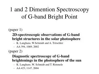
1 and 2 Dimention Spectroscopy of G-band Bright Point (paper 1) 2D-spectroscopic observations of G-band bright structures in the solar photosphere • K. Langhans, W.Schmidt and A. Tritschler • AA 394, 1069, 2002 (paper 2) Diagnostic spectroscopy of G-band brightenings in the photosphere of the sun • K. Langhans, W. Schmidt and T. Rimmele • AA 423, 1147, 2004
1. Introduction • G-band • 430nm • electronic transitions of the CH molecule FeII (430.32nm) CH (430.34nm)
B Optical surface Hot wall G-band White light GBP 1. Introduction • G-band bright points (GBP) • magnetic flux tube • Hot wall effect • Radiative heating • Photo-dissociation of the CH molecule by UV (?)
1. Introduction • Bright Point Index (BPI) • Two type of G-band Bright Point • An increased local continuum intensity small BPI • Difference in CH and FeII line depression large BPI I cont … continuum intensity at 430.33nm I Felc … line core intensity of FeII (430.32nm) I CHlc … line core intensity of CH (430.32nm) brackets … spatial average over a reference region
reference region line profile G-band image 30 x 30 arcsec large BPI small BPI dashed line … reference region
2. Observation (paper 1) • German Vacuum Tower Telescope • in Observatorio del Teide, Tenerife • Triple Etalon Solar Spectrometer (TESOS) • A single data set consists of 34 filtergrams • Wavelength step width : 1.62pm • Cadence : 17sec for the whole scan • FOV: 30 x 30 arcsec • August 4, 2001 10:27UT • S8.3W3.3
2. Observation (paper 2) • Richard B. Dunn Solar Telescope (DST) • in National Solar Observatory (NSO), SacPeak • Horizontal Spectrograph (HSG) with AO • FOV: 40 x 10.5 arcsec • October 6, 2001 • N20.2W12.3
3. Results (paper 1) (a) broadband at 431.1nm (b) narrowband continuum at 430.33nm (c) velocity map (FeII) • due to an increase of the local continuum intensity small BPI • due to a significant difference in CH and FeII line depression large BPI • located in downflow region
3. Results (paper 1) (d) CH-line core intensity (e) FeII-line core intensity (f) Bright Point Index • due to an increase of the local continuum intensity small BPI • due to a significant difference in CH and FeII line depression large BPI • located in downflow region
3. Results (paper 1) upflow downflow only data with BPI > 0.2 Center-of-gravity plot for each BPI bin The BPI is directory correlated with the downflow velocity
3. Results (paper 1) Plot for C G-band >= 0.1 Change in line depression = G2 is related to large BPI value
slit arcsec G-band image (broadband 1 nm at 430.5 nm, slit jaw camera) white light image (broadband 10 nm at 480 nm) Fig. 1. Broadband data.
exposures of high quality used for analysis. region around tracking point of AO Fig. 2. Spectral data. Example for one scan. a) Continuum intensity at 430.41 nm, b)–e) Line core intensities of the analyzed absorption lines.
4. Resuts (paper 2) Table 2. Averaged properties of bright points, based on the spectral data (Int.: interior; Surr.: surroundings; Ref.: reference). • 46 bright points were identified in the 3 scans • Continuum contrast at 430.41nm of interior and surroundings are almost equal line effect • Line depression CH
(2) (3) (1) • Typical intergranular bright point • At the edge of a granule • At the edge of a pore (2g) (3g) (1e) (3f)
(4) (5) (6) (4) The largest (5) Unclear GBPs (6) Bright but not GBP (6g) (6h) (4f) (6f)
4. Resuts (paper 2) course of the BPI (solid curve) and the G-band intensity contrast (dashed curve) velocity measurements (solid – CH, dashed – Fe I, dashed-dotted – Fe II) (a) … typical GBP in downflow region (b)(c)(d) … upflow velocity at GBP
granules GBPs Comparison of results for paper 1 and 2
granules GBPs Comparison of results for paper 1 and 2
down granules GBPs up Comparison of results for paper 1 and 2
5. Discussion • Upflows in magnetic elements? • Previous results … down flow of magnetic elements • Our results … Net downflows and upflows in individual bright points • Convective collapse rebound and result in upward propagating shocks • Flux tube with weak field strangths are unstable either a downflow or an upflow
Fig. 7. Comparison of selected properties derived from synthetic spectra to observables. The bars indicate the range of values, observed for the bright point interior. Data points shifted to the left (thick symbols) refer to the CH line, data points shifted to the right (thin symbols) to Fe II and the centered symbols refer to Fe I.
Table 3. Top: continuum contrasts, Ccont, derived from synthetic spectra, with respect to the FAL C-model atmosphere. The listed values from observation refer to the average (maximum) over all observed bright point interiors with respect to the spectrum of the reference region. Bottom: filling factors derived from Eqs. (3) and (4).
2. Observation (paper 2) Table 1. Top: specification of the spectral data. Bottom: specification of the image data.Abbreviations: FF – Flat Field, SNR – Signal-to-Noise Ratio.
Fig. 4. Illustration of the velocity measurements. Vertical dashed lines indicate the borders of bright point interior and immediate surroundings, respectively. Top: BPI. Bottom left: intensity contrast, continuum intensity (solid), integrated G-band intensity (dashed). Bottom right: flow velocity.