Download
1 / 17
170 likes | 238 Vues
Discovering the applications and implications of Green's Theorem in vector fields, showcasing calculations and proofs in different regions. Utilizes line integrals and double integrals for area calculations.

E N D
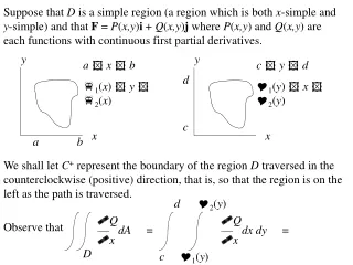
Suppose that D is a simple region (a region which is both x-simple and y-simple) and that F = P(x,y)i + Q(x,y)j where P(x,y) and Q(x,y) are each functions with continuous first partial derivatives. y y a x b 1(x) y 2(x) c y d 1(y) x 2(y) d c x x a b We shall let C+ represent the boundary of the region D traversed in the counterclockwise (positive) direction, that is, so that the region is on the left as the path is traversed. d 2(y) Q — dA = x Q — dx dy = x Observe that D c 1(y)
F = P(x,y)i + Q(x,y)j y y a x b 1(x) y 2(x) c y d 1(y) x 2(y) d c x x a b d 2(y) Q — dA = x Q — dx dy = x Observe that D c 1(y) d d 2(y) Q(x,y) dy = Q(2(y) , y) – Q(1(y) , y) dy = x = 1(y) c c
F = P(x,y)i + Q(x,y)j y y a x b 1(x) y 2(x) c y d 1(y) x 2(y) d c x x a b d Q(2(y) , y) – Q(1(y) , y) dy = c d d Q(2(t) , t) dt– Q(1(t) , t) dt = c c
F = P(x,y)i + Q(x,y)j y y a x b 1(x) y 2(x) c y d 1(y) x 2(y) d c x x a b d d Q(2(t) , t) dt– Q(1(t) , t) dt = c c d d (Q(2(t) , t)j) • (2(t) , 1) dt– (Q(1(t) , t)j) • (1(t) , 1) dt = c c Note that this line integral is over the right half of C in the counterclockwise direction. Note that this line integral is over the left half of C in the clockwise direction.
F = P(x,y)i + Q(x,y)j y y a x b 1(x) y 2(x) c y d 1(y) x 2(y) d c x x a b d d Q(2(t) , t) dt– Q(1(t) , t) dt = c c d d (Q(2(t) , t)j) • (2(t) , 1) dt– (Q(1(t) , t)j) • (1(t) , 1) dt = c c Q(x,y)j • ds C+
F = P(x,y)i + Q(x,y)j y y a x b 1(x) y 2(x) c y d 1(y) x 2(y) d c x x a b Q — dA = x We see then that Q(x,y)j • ds . D C+ P — dA = y Similarly, we find – P(x,y)i • ds . D C+
F = P(x,y)i + Q(x,y)j y y a x b 1(x) y 2(x) c y d 1(y) x 2(y) d c x x a b Q — dA – x P — dA = y Q(x,y)j • ds + P(x,y)i • ds . D D C+ C+ QP — – — dA = xy (P(x,y)i + Q(x,y)j) • ds = F • ds . D C+ C+
F = P(x,y)i + Q(x,y)j y y a x b 1(x) y 2(x) c y d 1(y) x 2(y) d c x x a b This proves Green’s Theorem (Theorem 1 on page 522) which can be stated as follows: Note that this is what we have called the scalar curl of F QP — – — dA = xy P dx + Q dy . F • ds = D C+ C+ Note: Green’s Theorem can be extended to a region which is not a simple region but can be partitioned into several simple regions.
Example Let F(x,y) = yi–xj and let C represent the circle of radius a centered at the origin and traversed counterclockwise. (a) Find using the definition of a line integral. F • ds C First, we parametrize C with (a cos t , a sin t) for 0 t 2 . 2 F • ds = F(c(t)) • c(t) dt = C 0 2 (a sin t , –a cos t) • (–a sin t , a cos t ) dt = – 2a2 0
(b) Find by using Green’s Theorem to write the line integral as a double integral, and evaluating this double integral. F • ds C Since F(x,y) = yi–xj , then we let P(x,y) = and Q(x,y) = From Green’s Theorem, we have y –x QP — – — dx dy = xy (– 1 – 1) dx dy = F • ds = C D D where D is the disk of radius a centered at the origin – 2 dx dy = – 2 dx dy = – 2(area of D) = – 2a2 D D
By applying Green’s Theorem with the vector field F = P(x,y)i + Q(x,y)j with P(x,y) = – y /2 and Q(x,y) = x / 2, we can find the area of a region D in R2 (as stated in Theorem 2 on page 524), because QP — – — dA = xy 1 1 — + — dA = 2 2 dx dy = D D D (area of D). In other words, we have that (area of D) = F • ds where C C is the boundary of D traversed in the counterclockwise direction, and F = (– y /2)i + (x / 2)j
Example Consider the area in the xy plane inside the graph of x2/3 + y2/3 = a2/3 (where a > 0 is a known constant). (a) Sketch a graph of this area. y (0 , a) (a , 0) (– a , 0) x (0 , – a)
(b) Write a double integral using rectangular coordinates to obtain the area, and write a double integral using polar coordinates to obtain the area. Observe how difficult evaluating each of these integrals will be. (a2/3– x2/3)3/2 a 2 a / (cos2/3 + sin2/3)3/2 dy dx r dr d – a – (a2/3– x2/3)3/2 0 0
(c) Use Green’s Theorem to obtain the area. First, we parametrize the curve which is the boundary of D by Then, by letting F = (– y /2)i + (x / 2)j , the area bounded by the curve is C() = ( a cos3 , a sin3 ) for 0 2 F • ds = C 2 1 — 2 (– a sin3 , a cos3 ) • (– 3a cos2 sin , 3a sin2 cos) d = 0 2 1 — 2 – (a sin3)(– 3a cos2 sin) + (a cos3 )(3a sin2 cos) d = 0
2 2 3 —a2 2 3 —a2 2 sin4 cos2 + sin2 cos4 d = sin2 cos2d = 0 0 2 2 2 1 – cos4 ———— d = 8 – (1/4)sin4 —————— = 8 3 —a2 2 3 —a2 2 sin22 ——— d = 4 3 —a2 2 0 0 0 Recall the half-angle and double-angle formulas which give us the following trig identities: 2 — = 8 3 —a2 2 3 — a2 8 1 sin cos = — sin(2) 2 1 sin2 = — (1 – cos(2)) 2
y Note: If (a, b) is a non-zero vector in R2, then any vector which is orthogonal to, and to the right of, (a, b) must be a positive multiple of ( , ) b – a (a, b) (b, – a). x Suppose that D is a simple region (a region which is both x-simple and y-simple) and that the closed path along the border of D in the counterclockwise direction, sometimes denoted as D, is parametrized by c(t) = (x(t) , y(t)). At any point along the path, an “outward” normal vector must be one which is orthogonal to the velocity vector c/(t) = (x/(t) , y/(t)). That is, an “outward” normal vector must be one which is a positive multiple of y (y/(t) , – x/(t)) (x/(t) , y/(t)) D x (y/(t) , – x/(t)).
Suppose F = P(x,y)i + Q(x,y)j is a vector field defined on D. Recall Green’s Theorem (Theorem 1 on page 522): QP — – — dA = xy F • ds D D Define the vector field V = – Q(x,y)i+P(x,y)j on D, and observe that V • c/(t) = V • (x/(t) , y/(t)) = Applying Green’s Theorem with the vector field V, we have – Q(x,y) x/(t) +P(x,y) y/(t) = F • (y/(t) , – x/(t)) PQ — + — dA = xy where n is understood to be the outward normal to D V • ds = F • nds D D D div(F) This proves the Divergence Theorem in the Plane (Theorem 4, page 527)