Electromagnetic Force
Electromagnetic Force. The electromagnetic force is given by Lorentz Force Equation ( After Dutch physicist Hendrik Antoon Lorentz (1853 – 1928)).

Electromagnetic Force
E N D
Presentation Transcript
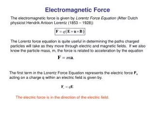
Electromagnetic Force The electromagnetic force is given by Lorentz Force Equation (After Dutch physicist Hendrik Antoon Lorentz (1853 – 1928)) The Lorentz force equation is quite useful in determining the paths charged particles will take as they move through electric and magnetic fields. If we also know the particle mass, m, the force is related to acceleration by the equation The first term in the Lorentz Force Equation represents the electric force Fe acting on a charge q within an electric field is given by. The electric force is in the direction of the electric field.
Magnetic Force The second term in the Lorentz Force Equation represents magnetic force Fm(N) on a moving charge q(C) is given by where the velocity of the charge is u (m/sec) within a field of magnetic flux density B (Wb/m2). The units are confirmed by using the equivalences Wb=(V)(sec) and J=(N)(m)=(C)(V). The magnetic force is at right angles to the magnetic field. The magnetic force requires that the charged particle be in motion. It should be noted that since the magnetic force acts in a direction normal to the particle velocity, the acceleration is normal to the velocity and the magnitude of the velocity vector is unaffected. Since the magnetic force is at right angles to the magnetic field, the work done by the magnetic field is given by
Magnetic Force D3.10: At a particular instant in time, in a region of space where E = 0 and B = 3ay Wb/m2, a 2 kg particle of charge 1 C moves with velocity 2ax m/sec. What is the particle’s acceleration due to the magnetic field? Given: q= 1 nC, m = 2 kg, u = 2 ax (m/sec), E = 0, B = 3 ay Wb/m2. Lorentz Force Equation Newtons’ Second Law Equating To calculate the units: P3.33: A 10. nC charge with velocity 100. m/sec in the z direction enters a region where the electric field intensity is 800. V/m ax and the magnetic flux density 12.0 Wb/m2ay. Determine the force vector acting on the charge. Given: q= 10 nC, u = 100 az (m/sec), E = 800 ax V/m, B = 12.0 ay Wb/m2.
Magnetic Force on a current Element Consider a line conducting current in the presence of a magnetic field. We wish to find the resulting force on the line. We can look at a small, differential segment dQ of charge moving with velocity u, and can calculate the differential force on this charge from velocity The velocity can also be written segment Therefore Now, since dQ/dt (in C/sec) corresponds to the current I in the line, we have (often referred to as the motor equation) We can use to find the force from a collection of current elements, using the integral
Magnetic Force – An infinite current Element Let’s consider a line of current I in the +az direction on the z-axis. For current element IdLa, we have The magnetic flux density B1 for an infinite length line of current is We know this element produces magnetic field, but the field cannot exert magnetic force on the element producing it. As an analogy, consider that the electric field of a point charge can exert no electric force on itself. What about the field from a second current element IdLb on this line? From Biot-Savart’s Law, we see that the cross product in this particular case will be zero, since IdL and aR will be in the same direction. So, we can say that a straight line of current exerts no magnetic force on itself.
a = -ax ρ = y Magnetic Force – Two current Elements Now let us consider a second line of current parallel to the first. The force dF12 from the magnetic field of line 1 acting on a differential section of line 2 is The magnetic flux density B1 for an infinite length line of current is recalled from equation to be By inspection of the figure we see that ρ = y and a = -ax. Inserting this in the above equation and considering that dL2 = dzaz, we have
a = -ax ρ = y Magnetic Force on a current Element To find the total force on a length L of line 2 from the field of line 1, we must integrate dF12 from +L to 0. We are integrating in this direction to account for the direction of the current. This gives us a repulsive force. Had we instead been seeking F21, the magnetic force acting on line 1 from the field of line 2, we would have found F21 = -F12. Conclusion: 1) Two parallel lines with current in opposite directions experience a force of repulsion. 2) For a pair of parallel lines with current in the same direction, a force of attraction would result.
Magnetic Force on a current Element In the more general case where the two lines are not parallel, or not straight, we could use the Law of Biot-Savart to find B1 and arrive at This equation is known as Ampere’s Law of Force between a pair of current carrying circuits and is analogous to Coulomb’s law of force between a pair of charges.
Magnetic Force D3.11: A pair of parallel infinite length lines each carry current I = 2A in the same direction. Determine the magnitude of the force per unit length between the two lines if their separation distance is (a) 10 cm, (b)100 cm. Is the force repulsive or attractive? (Ans: (a) 8 mN/m, (b) 0.8 mN/m, attractive) Magnetic force between two current elements when current flow is in the same direction Magnetic force per unit length Case (a) y = 10 cm Case (a) y = 10 cm
Magnetic Materials We know that current through a coil of wire will produce a magnetic field akin to that of a bar magnet. We also know that we can greatly enhance the field by wrapping the wire around an iron core. The iron is considered a magnetic material since it can influence, in this case amplify, the magnetic field. Relative permeabilities for a variety of materials. The degree to which a material can influence the magnetic field is given by its relative permeability,r, analogous to relative permittivityr for dielectrics. In free space (a vacuum), r = 1 and there is no effect on the field.
Magnetic Flux Density In the presence of an external magnetic field, a magnetic material gets magnetized (similar to an iron core). This property is referred to as magnetization M defined as where m (“chi”) is the material’s magnetic susceptibility. The total magnetic flux density inside the magnetic material including the effect of magnetization M in the presence of an external magnetic field H can be written as Substituting Where where is the material’s permeability, related to free space permittivity by the factor r, called the relative permeability.
Magnetostatic Boundary Conditions Will use Ampere’s circuital law and Gauss’s law to derive normal and tangential boundary conditions for magnetostatics. Ampere’s circuit law: Path 1 Path 4 Path 2 The current enclosed by the path is Path 3 We can break up the circulation of H into four integrals: Path 1: Path 2:
Magnetostatic Boundary Conditions Path 3: Path 4: Now combining our results (i.e., Path 1 + Path 2 + Path 3 + Path 4), we obtain ACL: Equating Tangential BC: A more general expression for the first magnetostatic boundary condition can be written as where a21 is a unit vector normal going from media 2 to media 1.
Magnetostatic Boundary Conditions Special Case: If the surface current density K = 0, we get If K = 0 The tangential magnetic field intensity is continuous across the boundary when the surface current density is zero. Important Note: (or) We know that Using the above relation, we obtain Therefore, we can say that The tangential component of the magnetic flux density B is not continuous across the boundary.
Magnetostatic Boundary Conditions Gauss’s Law for Magnetostatic fields: To find the second boundary condition, we center a Gaussian pillbox across the interface as shown in Figure. We can shrink h such that the flux out of the side of the pillbox is negligible. Then we have Normal BC:
Magnetostatic Boundary Conditions Normal BC: Thus, we see that the normal component of the magnetic flux density must be continuous across the boundary. Important Note: We know that Using the above relation, we obtain Therefore, we can say that The normal component of the magnetic field intensity is not continuous across the boundary (but the magnetic flux density is continuous).
Magnetostatic Boundary Conditions Example 3.11: The magnetic field intensity is given as H1 = 6ax + 2ay + 3az (A/m) in a medium with r1 = 6000 that exists for z < 0. We want to find H2 in a medium with r2 = 3000 for z >0. Step (a) and (b): The first step is to break H1 into its normal component (a) and its tangential component (b). Step (c): With no current at the interface, the tangential component is the same on both sides of the boundary. Step (d): Next, we find BN1 by multiplying HN1 by the permeability in medium 1. Step (e): This normal component B is the same on both sides of the boundary. Step (f): Then we can find HN2 by dividing BN2 by the permeability of medium 2. Step (g): The last step is to sum the fields .