Download
1 / 22
220 likes | 384 Vues
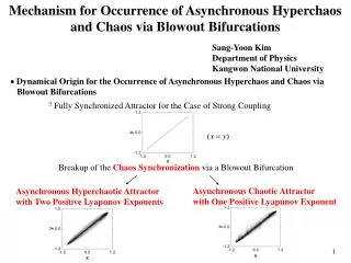
Mechanism for Occurrence of Asynchronous Hyperchaos and Chaos via Blowout Bifurcations. Dynamical Origin for the Occurrence of Asynchronous Hyperchaos and Chaos via Blowout Bifurcations. Sang-Yoon Kim Department of Physics Kangwon National University.

E N D
Mechanism for Occurrence of Asynchronous Hyperchaos and Chaos via Blowout Bifurcations Dynamical Origin for the Occurrence of Asynchronous Hyperchaos and Chaos via Blowout Bifurcations Sang-Yoon Kim Department of Physics Kangwon National University Fully Synchronized Attractor for the Case of Strong Coupling Breakup of the Chaos Synchronization via a Blowout Bifurcation Asynchronous Chaotic Attractor with One Positive Lyapunov Exponent Asynchronous Hyperchaotic Attractor with Two Positive Lyapunov Exponents
Two Coupled Logistic Maps (Representative Model) N Globally Coupled 1D Maps Reduced Map Governing the Dynamics of a Two-Cluster State Two-Cluster State Reduced 2D Map Globally Coupled Maps with Different Coupling Weight p (N2/N): “coupling weight factor” corresponding to the fraction of the total population in the 2nd cluster =0 Symmetric Coupling Case Occurrence of Asynchronous Hyperchaos =1 Unidirectional Coupling Case Occurrence of Asynchronous Chaos Investigation of the Consequence of the Blowout Bifurcation by varying from 0 to 1.
Transverse Stability of the Synchronous Chaotic Attractor (SCA) • Longitudinal Lyapunov Exponent of the SCA • Transverse Lyapunov Exponent of the SCA a=1.97, s=0.23 One-Band SCA on the Invariant Diagonal Transverse Lyapunov exponent For s>s* (=0.2299), <0 SCA on the Diagonal Occurrence of the Blowout Bifurcation for s=s* • SCA: Transversely Unstable (>0) for s<s* • Appearance of a New Asynchronous Attractor a=1.97
Type of Asynchronous Attractors Born via a Blowout Bifurcation New Coordinates For the accuracy of numerical calculations, we introduce new coordinates: SCA on the invariant v=0 line Transverse Lyapunov exponent of the SCA a=1.97, s=0.23 a=1.97 • Appearance of an Asynchronous Attractor through a Blowout Bifurcation of the SCA • The Type of an Asynchronous Attractor is Determined by the Sign of its 2nd Lyapunov Exponent2 (2 > 0 Hyperchaos, 2 < 0 Chaos) [ In the system of u and v, we can follow a trajectory until its length L becomes sufficiently long (e.g. L=108) for the calculation of the Lyapunov exponents of an asynchronous attractor.]
Computation of the Lyapunov Exponents 1 and 2 for a Trajectory Segment with Length L Evolution of a Set of Two Orthonormal Tangent Vectors under the Linearized Map Mn [DT(zn), zn (un,vn)]. • Reorthonormalization by the Gram-Schmidt Reorthonormalization Method (Direction of the 1st Vector: Unchanged) ( Has Only the Component Orthogonal to ) • 1st and 2nd Lyapunov Exponents 1 and 2
Second Lyapunov Exponent of the Asynchronous Attractor (: =0, : =0.852, : =1) a=1.97, L=108 Threshold Value * ( ~ 0.852) s.t. • < * Asynchronous Hyperchaotic Attractor (HCA) with 2 > 0 • > * Asynchronous Chaotic Attractor (CA) with 2 < 0 (dashed line: transverse Lyapunov exponent of the SCA) HCA for = 0 CA for = 1 a = 1.97 s = -0.0016 1 = 0.6087 2 = 0.0024 a = 1.97 s = -0.0016 1 = 0.6157 2 = -0.0028
Mechanism for the Occurrence of Asynchronous Hyperchaos and Chaos ’ Intermittent Asynchronous Attractor Born via a Blowout Bifurcation d = |v|: Transverse Variable d*: Threshold Value s.t. d < d*: Laminar Component (Off State), d > d*: Bursting Component (On State). d (t) We numerically follow a trajectory segment with large length L (=108), and calculate its 2nd Lyapunov exponent. • Decomposition of the 2nd Lyapunov Exponent 2of the Asynchronous Attractor : Weighted 2nd Lyapunov Exponent for the Laminar (Bursting) Component Fraction of the Time Spent in the i Component (Li: Time Spent in the i Component) 2nd Lyapunov Exponent of the i Component (primed summation is performed in each i component)
Competition between the Laminar and Bursting Components Laminar Component (: =0, : =0.852, : =1) a=1.97, d*=10-5 Bursting Component Sign of 2 : DeterminedviatheCompetitionoftheLaminarandBurstingComponents Threshold Value * (~ 0.852) s.t. Asynchronous Hyperchaotic Attractor with 2 > 0 < * > * Asynchronous Chaotic Attractor with 2 < 0
Effect of the Threshold Value d* on (: d*=10-6, : d*=10-8, : d*=10-10) a=1.97 •: Dependent on d* As d* Decreases, a Fraction of the Old Laminar Component is Transferred to the New Bursting Component: In the limit d*0, •2 Depends Only on the Difference Between the Strength of the Laminar and Bursting Components. The Conclusion as to the Type of Asynchronous Attractors is Independent of d*.
Blowout Bifurcations in High Dimensional Invertible Systems System: Coupled Hénon Maps New Coordinates: • Type of Asynchronous Attractors Born via Blowout Bifurcations (s*=0.787for b=0.1 and a=1.83) L=108 d*=10-4 d*=10-4 (: =0, : =0.905, : =1) Threshold Value * ( 0.905) s.t. For < * HCA with 2 > 0, for > * CA with 2 < 0.
1 0.4340 2 0.0031 1 0.4406 2 -0.0024 HCA for = 0 CA for = 1 a=1.83, s=-0.0016 a=1.83, s=-0.0016 System: Coupled Parametrically Forced Pendulums New Coordinates:
1 0.628 2 0.017 1 0.648 2 -0.008 • Type of Asynchronous Attractors Born via Blowout Bifurcations (s*=0.324for=1.0, =0.5, and A=0.85) L=107 d*=10-4 d*=10-4 (: =0, : =0.84, : =1) Threshold Value * ( 0.84) s.t. For < * HCA with 2 > 0, for > * CA with 2 < 0. HCA for = 0 CA for = 1 A=0.85 s=-0.006 A=0.85 s=-0.005
Summary • Mechanism for the Occurrence of the Hyperchaos and Chaos via Blowout Bifurcations Sign of the 2nd Lyapunov Exponent of the Asynchronous Attractor Born via a Blowout Bifurcation of the SCA: Determined via the Competition of the Laminar and Bursting Components Occurrence of the Hyperchaos Occurrence of the Chaos • Similar Results: Found in High-Dimensional Invertible Period-Doubling Systems such as Coupled Hénon Maps and Coupled Parametrically Forced Pendula
2q q q q q Effect of Asynchronous UPOs on the Bursting Component Change in the Number of Asynchronous UPOs with respect tos (from the first transverse bifurcation point st to the blow-out bifurcation point s*) •Symmetric Coupling Case (=0) (Period q=11) • Transverse PFB of a Synchronous Saddle • Asynchronous PDB
q q 2q q q q •Unidirectional Coupling Case (=1) (Period q=11) • Asynchronous SNB • Transverse TB • Asynchronous PDB
q q 2q 2q q q q q • Change in the Number of Asynchronous UPOs at the Blow-Out Bifurcation Point s* (=0.190) with respect to (Period q=11, Ns: No. of Saddles, Nr: No. of Repellers) • SNB • Reverse SNB • PDB • Reverse PDB
Transition from Chaos to Hyperchaos a=1.83 s=0.155 =1 1 0.478 2 0.018 For s = s* ( 0.163), a Transition from Chaos to Hyperchaos Occurs.
Characterization of the On-Off Intermittent Attractors Born via Blow-Out Bifurcations d: Transverse Variable (Denoting the Deviation from the Diagonal) d < d*: Laminar State (Off State) dd*: Bursting State (On State) p=p*: Blow-Out Bifurcation Point • Distribution of the Laminar Length: • Scaling of the Average Laminar Length: • Scaling of the Average Bursting Amplitude:
Phase Diagrams in Coupled 1D Maps System: Coupled 1D Maps: Dissipative Coupling Case with g(x, y) = f(y) – f(x) • Periodic Synchronization Symmetric Coupling (=0) Unidirectional Coupling (=1) Horizontal Lines: Longitudinal Bifurcations Synchronous Period-Doubling Bifurcations, Nonhorizontal Solid and Dashed Lines: Transverse Bifurcations (Solid Lines: Period-Doubling Bifurcations. Dashed Lines for =0 and 1: Pitchfork and Transcritical Bifurcations, Respectively.)
• Chaotic Synchronization Unidirectional Coupling (=1) Symmetric Coupling (=0) Hatched Region: Strong Synchronization, Light Gray Region: Bubbling, Dark Gray Region: Riddling Solid or Dashed Lines: First Transverse Bifurcation Lines (Solid Lines: Period-Doubling Bifurcations. Dashed Lines for =0 and 1: Pitchfork and Transcritical Bifurcations, Respectively.) Solid Circles: Blow-Out Bifurcation
Inertial Coupling Case with g(x, y) = y – x • Periodic Synchronization Unidirectional Coupling (=1) Symmetric Coupling (=0) Horizontal Lines: Longitudinal Bifurcations Synchronous Period-Doubling Bifurcations, Nonhorizontal Solid and Dashed Lines: Transverse Bifurcations (Solid Lines: Period-Doubling Bifurcations. Dashed Lines for =0 and 1: Pitchfork and Transcritical Bifurcations, Respectively.)
• Chaotic Synchronization Symmetric Coupling (=0) Unidirectional Coupling (=1) Hatched Region: Strong Synchronization, Light Gray Region: Bubbling, Dark Gray Region: Riddling Solid or Dashed Lines: First Transverse Bifurcation Lines (Solid Lines: Period-Doubling Bifurcations. Dashed Lines for =0 and 1: Pitchfork and Transcritical Bifurcations, Respectively.) Solid Circles: Blow-Out Bifurcation