Download
1 / 24
240 likes | 413 Vues
Challenges in the Measurement of Neutron Star Radii. Cole Miller University of Maryland. Collaborators: Romain Artigue , Didier Barret , Sudip Bhattacharyya, Stratos Boutloukos , Novarah Kazmi , Fred Lamb, Ka Ho Lo. Outline. NS masses are known up to 2 M sun . What about radii?.

E N D
Challenges in the Measurement of Neutron Star Radii Cole Miller University of Maryland Collaborators: RomainArtigue, Didier Barret, Sudip Bhattacharyya, StratosBoutloukos, Novarah Kazmi, Fred Lamb, Ka Ho Lo
Outline NS masses are known up to 2 Msun. What about radii? • Radii from X-ray bursts • Radii from cooling neutron stars • Radii from X-ray light curves • The promise of gravitational waves Key point: all current NS radius estimates are dominated by systematics. None are reliable. But hope exists for the future.
Measuring stellar radii • Ordinary star, like the Sun • Too far for angular resolution • But can get luminosity L • If we assume blackbody, R2=L/(4psT4) • But for NS, usually gives ~5 km! • Why? Spectral shape is ~Planck, but inefficient emission • Need good spectral models • But data usually insufficient to test
M and R from X-ray Bursts • van Paradijs(1979) method • XRB: thermonuclear explosions on accreting NS • Assume known spectrum, emission over whole surf. • Only with RXTE (1995-2011) is there enough data http://cococubed.asu.edu/images/binaries/images/xray_burst3_web.jpg
4U 1820 Bursts: Soft EOS? Guver et al. 2010; known dist (globular) Uses most optimistic assumption: no systematics, only statistical uncertainties But small errors are misleading; only ~10-8 of prior prob. space gives M, R in real numbers! (Guver et al., Steiner et al.) Spectral model is terriblefit to best data! • Fits of good spectral models to hours-long burstsshow that fraction of emitting area changes!
Inferred relative emitting areas, for 102 16-s segments near the peak of the 1820 superburst: Miller et al., in prep
Emission from Cooling NS • Old, transiently accreting NS • Deep crustal heating (e.g., e capture) • If know average accretion rate, emission provides probe of cooling; can we use to fit radius? • Predictions of simple model: Minimum level of emission Spectrum should be thermalNo variability: steady, slow decay
Cooling NS Observations • Oops! • All the predictions fail L sometimes below minimum Large power law component Significant variability • Excuses exist, but failure of basic model means we can’t use these observations to get R • Also: is surface mainly H? He? C? Makes 10s of percent difference to R • Magnetic field can also alter spectrum • Again, wide variety of models fit data, thus can’t use data to say which model is correct
RXJ 1856.5–3754 • Specific isolated NS • Argument: BB most efficient emitter, thus R>=RBB • True for bolometric but not for given band • Example: Ho et al. condensed surface fit • Different R constraints for different models Klähn et al. 2006
RXJ 1856.5–3754 • Specific isolated NS • Argument: BB most efficient emitter, thus R>=RBB • True for bolometric but not for given band • Example: Ho et al. condensed surface fit • Different R constraints for different models Klähn et al. 2006
Baryonic vs. Grav. Mass • Pulsar B in the double pulsar system • Mgrav=1.249+-0.001 Msun • If this came from e capture on Mg and Ne, Mbary=1.366-1.375 Msun for core • But what about fallback? • Or could mass be lost after collapse?
Ray Tracing and Light Curves • Rapidly rotating star 300-600 Hz vsurf~0.1-0.2c SR+GR effects • Light curve informative about M, R Bogdanov 2012; MSP • Must deal carefully with degeneracies • Lo et al., arXiv:1304.2330 (synth data); no systematic that gives good fit, tight constraints, and large bias Weinberg, Miller, and Lamb 2001
Phase Accumulation from GWs • aLIGO/Virgo: >=2015 • Deviation from point mass in NS-NS inspiral: accumulated tidal effects • For aLIGO, can measure tidal param(Del Pozzo+ 2013: distinguish R~11, 13 km?) • Recent analytics confirmed by numerical relativity (Bernuzzi et al. 2012) • High-freq sensitivity key Damour et al., arXiv:1203.4352 High-freq modeling, too
Conclusions Current radius estimates are all dominated by systematics Light curve fitting shows promise: No deviations we have tried from our models produce significant biases while fitting well and also giving apparently strong constraints. LOFT, AXTAR, NICER Future measurements of M and R using gravitational waves may be competitive in their precision with X-ray based estimates, and will have very different systematics Open question: how can we best combine astronomical information with laboratory measurements (e.g., 208Pb skin thickness)?
Ray Tracing from MSP • S. Bogdanov 2012 • Binary millisecond pulsar J0437-4715 • Two spots, H atm • Multitemp plus Comptonizedspect • Qs about beaming, spectrum; intriguing results, though! Bogdanov 2012
High inclinations allow tight constraints on M and R Spot and observer inclinations = 90°, high background
Low inclinations produce looser constraints Amplitude similar to the previous slide, but low spot and observer inclinations, low background
Independent knowledge of the observer’s inclination can increase the precision spot and observer inclinations = 90°, high background Observer inclination unknown
Independent knowledge of the observer’s inclination can increase the precision spot and observer inclinations = 90°, high background Observer inclination known to be 90°
Incorrect modeling of the spot shapeincreases the uncertainties spot and observer inclinations = 90°, medium background Actual spot elongated E-W by 45°
Fits Using New Models 64-second segment at peak temperature Yes! New models from Suleimanov et al. 2010 do seem to fit the data quite well. This model has F=0.95FEdd Best fit: 2/dof=42.3/48 Best B-E fit: 2/dof=55.6/50 For full 102-segment data set, best fit has 2/dof=5238/5098 B-E best: 2/dof=5770/4998 Fits are spectacularly good! Much better than B-E, so further info can be derived Pure He, log g = 14.3, F=0.95FEdd Model from Suleimanov et al. 2010
Keplerian Constraints Suppose we observe periodic variations in the radial velocity of star 1, with period Pb and amplitude vrad. Then we can construct the mass function This is a lower limit to the mass of star 2, but depends on the unknown inclination i and the unknown mass m1 of the observed star.
Post-Keplerian Parameters With high-precision timing, can break degeneracies: If both objects are pulsars, also get mass ratio. Allows mass measurements, GR tests
Artigue et al. 2013 Analysis of bursts from 4U 1636-536; previously claimedto contradict rotating spot model c2/dof for all five bursts combined: 1859/1850 (44%) c2/dof for far left burst only: 401.8/372 (14%) Hot spot model fits very well