Sarah Gibson
The calm before the storm: The link between quiescent cavities and CMEs. Sarah Gibson. David Foster, Joan Burkepile, Giuliana de Toma, Andy Stanger. AGU, Spring 2005. Sarah Gibson. Outline New, quantitative observational analysis of quiescent white light cavities Frequency Morphology


Sarah Gibson
E N D
Presentation Transcript
The calm before the storm: The link between quiescent cavities and CMEs Sarah Gibson David Foster, Joan Burkepile, Giuliana de Toma, Andy Stanger AGU, Spring 2005 Sarah Gibson
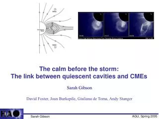
Outline • New, quantitative observational analysis of quiescent white light cavities • Frequency • Morphology • Intensity contrast • Correlations • Relation between quiescent cavities and CMEs • Relevance to structure of pre-CME coronal magnetic field Mauna Loa Mk4 white light coronagraph image showing quiescent cavity: November 18, 1999 CME eruption of cavity: November 19, 1999 Sarah Gibson AGU, Spring 2005
Magnetic flux ropes: What’s the attraction? • Theoretically compelling: • Coronal magnetic helicity very nearly conserved as a global quantity (Berger and Field, 1984) • Magnetically dominated plasma relaxes to minimum energy conserving helicity (Taylor, 1974, 1986) • Free energy stored in still-twisted magnetic fields is plausible CME driver (Low, 1999 ) • Flux ropes “fundamental building blocks of magnetism in the solar atmosphere”? (Rust, 2003) • Observationally compelling: • Magnetic flux ropes models have been applied to solar regimes from the interior out to 1 AU • Distinct observational signatures of flux ropes identify regions of stored magnetic energy • Evolution of these flux rope signatures clues to predicting eruptions?
Magnetic flux ropes What’s a magnetic flux rope? Suggested definition: A set of magnetic field lines winding about an axial field line in an organized manner Are there flux ropes in interplanetary space? Pretty well accepted Are there flux ropes in the corona during CME eruption? Also quite well accepted Do flux ropes exist quiescently in the corona prior to the CME? Controversial If they exist quiescently in the corona, are they formed from emerging twisted magnetic flux, or from photospheric motions? Controversial
Magnetic flux ropes Do flux ropes exist quiescently in the corona prior to the CME? Controversial
CMEs-3 part structure: Observations SOHO/LASCO C2/C3 white light coronagraphs (Illing and Hundhausen, 1986)
Uniting theme: Magnetic flux rope -- the question is, when does it form? CMEs-3 part structure: Models Low and Hundhausen, 1995 Linker et al., 2003 Krall et al., 2001 Lynch et al., 2004
Quiescent cavity-3 part structure NCAR/HAO Newkirk WLCC telescope, March 18 1988 eclipse, Philippines • Eclipse observations have long (as early as eclipse of Jan 22, 1898!) demonstrated the presence of non-eruptive 3 part structures -- prominence/cavity/helmet • Prominence cavity = filament channel viewed at limb • Prominence cavities also sometimes visible in H-a and radio (Straka et al., 1975; Kundu et al., 1979) as well as EUV (Sterling and Moore, 1997) and soft Xray (Serio et al., 1978; Hudson et al. 1999) • White light observations have some advantages • Only sensitive to density • Can see cavities higher above limb • Quantitative comparison to 3 part CME in white light possible
Innermost to outermost: EIT 284, Mark IV, Lasco C2, Lasco C3 Quiescent cavities occur in the low corona
Observational properties of cavities: Frequency • First noted all days November 1999 -- September 2004 where HAO/MLSO Mark IV coronagraph showed clear cavities: 206 days with clear cavities • Solar cycle effect -- more cavities visible during descending phase • Correlated with polar crown filament visibility • Lower limit on days with cavities -- many more identified if cavity systems examined in detail
Observational properties of cavities: Frequency Then chose most visible cases: 25 cavities
Observational properties of cavities: Frequency These are not independent cavities -- together represent 12 systems
Observational properties of cavities: Frequency In order to study evolution of systems, also analyzed adjacent days and reappearances as the system rotated past solar limbs: 88 cavities total quantitatively analyzed • Polar crown filament systems span more than four months • Cavities visible for as many as nine days
Observational properties of cavities: Morphology • (all values Minimum/Mean/Maximum, 12 system best only, full dataset of 88) • Cavity distance from equator: 5/56/77 5/56/90 degrees • Cavity width: 6/18/364/19/40 degrees • Cavity height: 1.25/1.47/1.601.24/1.46/1.64 Rsun
Observational properties of cavities: Contrast • (all values Minimum/Mean/Maximum 12 system best only, reduced dataset of 69) • Cavity intensity depletion at 1.2 Rsun: • Equatorward: 1 %/ 27% / 47%0 %/ 26% / 54% • Poleward:0 %/ 16% / 34%0 %/ 14% / 34% • Cavity sharpness (slope at edge): • Equatorward: 8.8e-9 / 2.5e-8 / 3.9e-82.1e-9 / 2.0e-8 / 6.7e-8 (Bsun/degree) • Poleward:1.7e-9 / 1.8e-8 / 4.2e-83.4e-10 / 1.4e-8 / 4.9e-8 (Bsun/degree) prominence
Observational properties of cavities: Correlations • Distance from equator vs. time follows streamer belt : • near equator around minimum • all latitudes during descending phase • Width vs. height: • Fatter tends to be taller • Intensity depletion vs. cavity sharpness: • darker tends to have sharper boundaries • Intensity depletion vs. width --Two conflicting effects: • Morphology -- parallel to line of sight ---> smaller, sharper boundary cavities • Evolution -- more “mature” filament cavities tend to be higher/fatter and sharper boundaries
CMEs from cavities Of the 12 systems: 3 were observed by MLSO Mark IV to erupt outwards in a CME at least once in their lifetime. Two of these were Polar Crown Filaments (PCFs) 5 more systems could be associated with CMEs observed by SOHO but at times of no Mark IV cavity data, either due to Mark IV not observing, or because the system was not near a limb. All but one of these were PCFs, the other was a high latitude CF. 4 systems could not be associated with CMEs. 2 was a PCF, 2 were not. Both PCF cases had a lot of missing data days around it, and at the times when it might be expected to be visible at the opposing limb. ..or to put it another way -- 9 out 12 were PCFs (or high latitude CFs) -- 7 of these erupted at some time, and the others had significant data dropouts for both Mark IV and SOHO.
Example of cavity --> CME: November 19, 1999 November 18, 1999
Example of cavity --> CME: February 5, 1999 February 4, 1999
CMEs from cavities Total of Mk4 observations of 6 cavities --> CMEs (one system had two cases, another had three, separated by a month or more). We then searched Mark IV observer’s logs for good 3-part CMEs, and examined data prior to these for precursor cavities. This gave us an additional 8 CMEs <-- cavities. How do the cavities-->CMEs differ from the CMEs<--cavities? Cavities --> CMEs -- PCFs, slower speeds • 5/6 were PCFs • Speed min/mean/max: 155/334/660 km/sec CMEs <-- cavities -- active region and some quite fast • 7/8 associated with (or at least near) AR • Speed: min/mean/max: 498 / 836 /1280 km/sec
Example of CME <-- cavity: August 9, 2001 August 8, 2001
Example of CME <-- cavity: May 15, 2001 Active region/Fast CME case! see Maricic et al., 2004 for detailed analysis
CMEs from cavities How are the cavities that erupt as CMEs distinguished from the general set of cavities? Historically, cases have been found where a quiescent cavity system was observed to gradually rise, swell, and ultimately be released in a CME (Fisher and Poland, 1988; Illing and Hundhausen, 1985; Hundhausen, 1999) This is part of the same phenomenon of streamers swelling before eruption (e.g. “bugles” in synoptic maps as pointed out by Hundhausen, 1993.) Also associated with a trend for filaments to be more likely to erupt in a CME if they extend high enough up in the corona (between 1.2 and 1.35 Rsun -- the lower bounds of the Mark IV coronagraph) (Munro, 1979; Gilbert et al., 2000)
CMEs from cavities • We therefore considered whether cavities • had filaments high enough to be seen in white light • exhibited “necking” Of the 10 cases where we had cavity observations within 24 hours of eruption: • 6 out of 10 had high filaments (vs. 25/99 of entire sample) • 10 out of 10 had necking (vs. 63/99 whole sample) • of these 7 out of 10 are truly bulging (vs. 27/99 whole sample) • 2 out of 10 are within error bars straight up and down (vs 36/99) • 0 out of 10 have no necking (vs 36/99)
CMEs from cavities There are also good examples of the height of the cavity, degree of necking, and presence/height of the filament increasing in the days leading up to the CME: July 21, 2002 July 22, 2002 (CME seen by LASCO early July 23, 2002)
CMEs from cavities …and in a system as a whole Oct 1 Oct 19 Nov 2 Nov 19 Dec 13 Dec 26 (CMEs Nov 19, Dec 31)
CMEs from cavities We also considered whether cavities erupting as CMEs were darker or had sharper boundaries than those that did not immediately erupt • No clear evidence that they are darker (min/mean/max polar-edge depletion = 4% / 16% / 43% vs. 1 %/ 14%/ 34% for non-CMEs) • May be more sharply defined (min/mean/max polar-edge slope = 8.6d-9 / 2.9d-8 / 1.1d-7 vs. 3.4d-10 / 1.3d-8 / 4.89d-8 for non-CMEs) • There are a few cases where depletion and especially sharpness may increase in the day or days leading up to the CME • These are preliminary results -- need more data!
Cavities are ubiquitous, and undersampled due to line of sight effects • Quite possibly whenever there is a filament channel, there is a filament cavity • Visibility depends upon morphology (particularly height), intensity contrast, and degree of obscuring features along the line of sight • STEREO will be essential to disentangling morphology vs. evolution effects! • Cavities are parts of filaments: • can extend higher than 1.6 solar radii • models of filament systems (particularly polar crown filaments) should consider observed properties of cavities White light quiescent cavities are biassed to Polar Crown Filament Systems • Extremely long-lived, and stable • The presence of a quiescent cavity is not by itself a good indicator of an impending CME • However, given enough time a PCF-cavity system will erupt, and probably more than once • A cavity that grows higher, more bulging (and/or contains a filament) and possibly more sharply defined is a good bet Small, non-PCF (even active region!) cavities do exist • We found some when we worked backwards from 3 part CMEs. • And finally -- we have demonstrated 3-part quiescent structures appear to erupt bodily as CMEs. CONCLUSIONS
So do observations imply a precursor magnetic flux rope? I say, yes! For three reasons: • Cavities can be formed by increased pressure of sheared, expanding fields • Flux ropes are certainly consistent with this • But so are other more generally sheared fields: and the presence of sheared fields prior to a CME is not controversial. • But cavities also exist for days/weeks/months -- what prevents the sheared field from refilling? • Detached fields of magnetic flux ropes will enhance cavity longevity, thermally isolating them andsuppressing their being refilled from below • Cavities have sharply defined, circular boundaries, and cavities-->CMEs exhibit necking • This is a natural consequence of an organized winding of field lines about axial field line (my definition of flux rope) • A sharp boundary is consistent with a magnetic flux surface at the outer boundary of a flux rope • Necking is consistant with a flux rope high enough in the corona to show its boundary at levels lower than its axis Which brings us back to magnetic flux ropes
Throwing down the gauntlet… The challenges for CMEs models, with or without pre-existing flux ropes, are: To reproduce cavity intensity contrast and sharp edges consistent with observations To reproduce cavity sizes (heights/widths/lengths) consistent with observations To reproduce cavity evolution (necking, high filament, sharpenimg boundary) prior to CME To reproduce cavity longevity (months!) and stability