Parallel Processing for Scientific Applications: Harnessing the Power of Multiple Processes
This lecture explores parallel computing as a method to tackle complex scientific problems through multiple processes. It demonstrates the necessity of parallel processing in areas such as numerical prototyping, climate prediction, and physical simulations, highlighting the challenges of modeling real phenomena. It discusses efficient algorithm design, scalability, and the architecture of parallel computers, including SMP and MPP systems. Case studies illustrate the computational demands of tasks like weather prediction and the efficiency required for processing vast amounts of data in parallel.


Parallel Processing for Scientific Applications: Harnessing the Power of Multiple Processes
E N D
Presentation Transcript
Parallel Computing Multiple processes cooperating to solve a single problem
Why Parallel Computing ? • Easy to get huge computational problems • physical simulation in 3D: 100 x 100 x 100 = 106 • oceanography example: 48 M cells, several variables per cell, one time step = 30 Gflop = 30,000,000,000 floating point operations)
Why Parallel Computing ? • Numerical Prototyping: • real phenomena are too complicated to model • real experiments are too hard, too expensive, or too dangerous for a laboratory: • Examples: simulate aging effects on nuclear weapon (ASCI Project), oil reservoir simulation, large wind tunnels, galactic evolution, whole factory or product life cycle design and optimization, DNA matching (bioinformatics)
Grid point An Example -- Climate Prediction
An Example -- Climate Prediction • What is Climate? • Climate (longitude, latitude, height, time) • return a vector of 6 values: • temperature, pressure, humidity, and wind velocity (3 words) • Discretize: only evaluate on a grid point; • Climate(i, j, k, n), where t = n*dt, dt is a fixed time step, n an integer, i,j,k are integers indexing the grid cells.
An Example -- Climate Prediction • Area: 3000 x 3000 miles, Height: 11 miles --- 3000x3000x11 cube mile domain • Segment size: 0.1x0.1x0.1 cube miles --1011 different segments • Two-day period, dt = 0.5 hours (2x24x2=96) • 100 instructions per segment • the computation of parameters inside a segment uses the initial values and the values from neighboring segments
An Example -- Climate Prediction • A single updating of the parameters in the entire domain requires 1011x100, or 1013 instructions (10 Trillion instructions). Update 96 times -- 1015instructions • Single-CPU supercomputer: • 1000 MHz RISC CPU • Execution time: 280 hours. • ??? Taking 280hours to predict the weather for next 48 hours.
Issues in Parallel Computing • Design of Parallel Computers • Design of Efficient Algorithms • Methods for Evaluating Parallel Algorithms • Parallel Programming Languages • Parallel Programming Tools • Portable Parallel Programs • Automatic Programming of Parallel Computers
Design of Parallel Computer • Parallel computingis information processing that emphasizes the concurrent manipulation of data elements belonging to one or more processes solving a single problem [Quinn:1994] • Parallel computer: a multiple-processor computer capable of parallel computing.
Efficient Algorithms • Throughput: the number of results per second • Speedup: S = T1 / Tp • Efficiency = S/P (P= no. of processor)
Scalability • Algorithmic scalability: an algorithm is scalable if the available parallelism increases at least linearly with problem size. • Architectural scalability: an architecture is scalable if it continues to yield the same performance per processor, as the number of processors is increased and as the problem size is increased. • Solve larger problems in the same amount of time by buying a parallel computer with more processors. ($$$$$ ??)
Parallel Architectures • SMP: Symmetric Multiprocessor (SGI Power Challenger, SUN Enterprise 6000) • MPP: Massively Parallel Processors • INTEL ASCI Red: 9152 processors (1997) • SGI/Cray T3E120 LC1080-512 1080 nodes (1998) • Cluster: True distributed systems -- tightly-coupled software on a loosely-coupled (LAN-based) hardware. • NOW: Network of Workstation or COW: Cluster of Workstations, Pile-of-PC (PoPC)
Levels of Abstraction Applications (Sequential ?) (Parallel ?) Programming Models (Shared Memory ?) (Message Passing ?) Hardware Architecture Addressing Space (Shared Memory?) (Distributed Memory ?)
A Simple Example • Take a paper and pen. • Algorithm: • Step 1: Write a number on your pad • Step 2: Compute the sum of your neighbor's values • Step 3: Write the sum on the paper
** Questions 1 How do you get values from your neighbors?
Shared Memory Model 5, 0, 4
Message Passing Model Hey !! What’s your number ?
** Questions 2 Are you sure the sum is correct ?
Some processor starts earlier 5+0+4 = 9
Synchronization Problem !! Step 3. 9 9+5+0=14 Step 2.
** Questions 3 How do you decide when you are done? (throw away the paper)
Some processor finished earlier 5+0+4 = 9
Some processor finished earlier Sorry !! We closed !!
Some processor finished earlier Sorry !! We closed !! ?+5+0=? Step 2.
1. Based on Control Mechanism • Flynn’s Classification : data or instruction stream : • SISD: single instruction stream single data streams • SIMD: single instruction stream multiple data streams • MIMD: multiple instruction streams multiple data streams • MISD: multiple instruction stream single data stream
SIMD • Examples: • Thinking Machines: CM-1, CM-2 • MasPar MP-1 and MP-2 • Simple processor: e.g., 1- or 4-bit CPU • Fast global synchronization (global clock) • Fast neighborhood communication • Applications: image/signal processing, numerical analysis, data compression,...
2. Based on Address-space organization • Bell’s Classification on MIMD architecture • Message-passing architecture • local or private memory • multicomputer = MIMD message-passing computer (or distributed-memory computer) • Shared-address-space architecture • hardware support for one-side communication (read/write) • multiprocessor = MIMD shared-address-space computers
Address Space • A region of a computer’s total memory within which addresses are continuous and may refer to one another directly by hardware. • A shared memorycomputer has only one user-visible address space • A disjoin memorycomputer can have several. • Disjoint memory is more commonly called distributed memory, but the memory of many shared memory computer (multiprocessors) is physically distributed.
Multiprocessors vs. Multicomputers • Shared-Memory Multiprocessors Models • UMA: uniform memory access (all SMP servers) • NUMA: nonuniform-memory-access (DASH, T3E) • COMA: cache-only memory architecture (KSR) • Distributed-Memory Multicomputers Model • message-passing network • NORMA model (no-remote-memory-access) • IBM SP2, Intel Paragon, TMC CM-5, INTEL ASCI Red, cluster
Parallel Computers at HKU CYC 807 • Symmetric Multiprocessors (SMPs) • SGI PowerChallenge • Cluster: • IBM PowerPC Clusters • Distributed Memory Machine • IBM SP2 CYC LG 102. Computer Center
Symmetric Multiprocessors (SMPs) • Processors are connected to a shared memory module through a shared bus • Each processor has equal right to access : • the shared memory • all I/O devices • A single copy of OS
32-bit address 64-bit data 533 MB/s P6 P6 P6 P6 Pentium Pro processor bus Memory controller 32-bit address 32-bit data 132 MB/s PCI Bridge DRAM Controller Data Path PCI Bus Mem data (72 bits) NIC PCI Device PCI Device MIC MIC MIC MIC Interleave data (288 bits) To Network Main memory (4 GB max.) Intel SMP MIC: memory interface controller CYC414 SRG Lab.
SMP Machine SGI POWER CHALLENGE • POWER CHALLENGE XL • 2-36 CPUs • 16 GB memory (for 36 CPUs) • The bus performance: up to 1.2GB/sec • Runs on a 64 bits OS (IRIX6.2) • Common memory is shared which suitable for single-address-space programming
Distributed Memory Machine • Consists of multiple computers (nodes) • Nodes are communicated by message passing • Each node is an autonomous computer • Processor(s) (may be an SMP) • Local memory • Disks, network adapter, and other I/O peripherals • No-remote-memory-access (NORMA)
Distributed Memory Machine IBM SP2 • SP2 => Scalable POWERparallel System • Developed based on RISC System/6000 workstation • Power 2 processor, 66.6 MHz, 266 MFLOP
Switch among the nodes simultaneously and quickly Maximum 40MB point-to-point bandwidth SP2 - High Performance Switch 8x8 Switch
SP2 - Nodes (POWER 2 processor) • Two types of nodes: • Thin node (smaller capacity, used to process individual works) 4 micro-channel slots, 96KB cache, 64-512MB memory, 1-4 GB disk • Wide node (larger capacity, used to be servers of the system) 8 micro-channel slots, 288KB cache, 64-2048MB memory, 1-8 GB disk
SP2 • The largest SP (P2SC, 120 MHz) machine: Pacific Northwest National Lab. U.S., 512 processors, TOP 26, 1998.
What’s a Cluster ? • A cluster is a group of whole computers that works cooperatively as a single system to provide fast and efficient computing service.
Cluster in Graduate Student Lab. Switched Ethernet I need variable A from Node 2! IBM PowerPC Cluster OK! Thank You! Node 1 Node 2 Node 3 Node 4 IBM PowerPC
Clusters • Advantages • Cheaper • Easy to scale • Coarse-grain parallelism • Disadvantages • Poor communication performance (typically the latency) as compared with other parallel systems
TOP 500 (1997) • TOP 1 INTEL: ASCI Red at Sandia Nat’l Lab. USA, June 1997 • TOP 2 Hitachi/Tsukuba:CP-PACS (2048 processors), 0.368 Tflops at Univ. Tsukuba Japan, 1996 • TOP 3 SGI/Gray: T3E 900 LC696-128 (696 processors), 0.264 Tflops at UK, Meteorological Office UK, 1997
TOP 500 (June, 1998) • TOP 1 INTEL: ASCI Red (9152 Pentium Pro processors, 200 MHz), 1.3 Teraflops at Sandia Nat’l Lab. U.S., since June 1997 • TOP 2 SGI/Gray: T3E 1200 LC1080-512, 1080 processors, 0.891 Tflops, U.S. government, 1998 installed • TOP 3. SGI/Cray: T3E900 LC1248-128, 1248 processors, 0.634 Tflops, U.S. government
INTEL ASCI Red Compute node: 4536 (Dual Pentium Pro 200 MHz sharing a 533 MB/s bus) • Peak speed.: 1.8 Teraflops (Trillion: 10 12) • 1,600 square feet 85 cabinets