Material Balance Equations
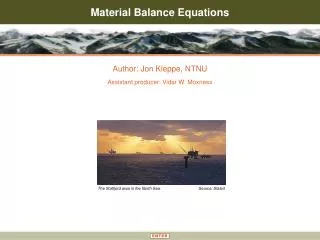
Material Balance Equations. The Statfjord area in the North Sea. Source: Statoil. Author: Jon Kleppe, NTNU. Assistant producer: Vidar W. Moxness. Introduction. INTRODUCTION. MODELLING. APPLICATION.

Material Balance Equations
E N D
Presentation Transcript
Material Balance Equations The Statfjord area in the North Sea. Source: Statoil Author: Jon Kleppe, NTNU Assistant producer: Vidar W. Moxness
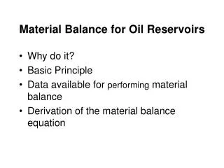
Introduction INTRODUCTION MODELLING APPLICATION To illustrate the simplest possible model we can have for analysis of reservoir behavior, we will start with derivation of so-called “Material Balance Equations”. This type of model excludes fluid flow inside the reservoir, and considers fluid and rock expansion/compression effects only, in addition, of course, to fluid injection and production. This module is meant to be an extra help to the lectures in “Reservoir recovery techniques” by giving examples to the curriculum covered by the handout “Material Balance Equations”. The structure of the model is shown below. • Learning goals • Basic understanding of material balance • The handout “Material Balance Equations” can be • downloaded from here: SUMMARY matbal.pdf Introduction Application Modelling Summary Block diagram Saturation Water influence Initial gascap Material conservation Equations Graph A Graph B Plot 1 Plot 2 Plot 3
Block diagram of a producing reservoir INTRODUCTION MODELLING Block diagram Material conservation Graph A B Equations Saturation The essence of material balance is described in the block diagram below. From the initial stage oil, gas & water is produced. At the same time gas & water is (re)injected into the reservoir to maintain pressure. There is also an influx from the aquifer below the reservoir. Due to change in pressure, the pore volume as well as the fraction of the volume occupied by gas, oil & water will change. APPLICATION SUMMARY Click to display symbols used
Amount of fluids pre sent Amount of Amount of fluids rem aining ì ü ì ü ì ü ï ï ï ï ï ï in the res ervoir ini tially - fluids pro duced = in the res ervoir fin ally í ý í ý í ý ï ï ï ï ï ï (st. vol. ) (st. vol. ) (st. vol. ) î þ î þ î þ Principle of material conservation INTRODUCTION MODELLING Block diagram Material conservation Graph A B Equations Saturation From the block diagram we get the expression below, which is the basis for the material balance formulas. APPLICATION SUMMARY • Note that “fluids produced” include all influence on the reservoir: • Production • Injection • Aquifer influx
Formation Volume Factor in the Black Oil model INTRODUCTION MODELLING Block diagram Material conservation Graph A B Equations Saturation The formation volume factors (FVF) tell how much the oil, gas and water is compressed at a given pressure. Bo = reservoir volume of oil / standard volume of oil Bg = reservoir volume of gas / standard volume of gas Bw = reservoir volume of water / standard volume of water The graphs below show how the FVF of oil, gas and water develop vs pressure. Click on the buttons to show the graphs. APPLICATION SUMMARY Bo vs. P Bg vs. P Bw vs. P Bo Bg Bw P P P Click to display symbols used
Solution Gas-Oil Ratio in the Black Oil model INTRODUCTION MODELLING Block diagram Material conservation Graph A B Equations Saturation The Rso plot shows how the solution gas ratio develops vs pressure. When the pressure reaches the bubblepointpressure, it is no longer possible to solve more gas into the oil. Thus the gradient of the curve becomes zero. Rs = standard volume gas / standard volume oil Click on the button below to see the typical pressure dependency of the solution gas-oil ratio in the black oil model. APPLICATION SUMMARY Rso vs. P Rso P Click to display symbols used
The complete black oil material balance equation INTRODUCTION MODELLING Block diagram Material conservation Graph A B Equations Saturation The final material balance relationships is given below. How these expressions are derived can be studied in the Material Balance pdf document. matbal.pdf APPLICATION SUMMARY Where: production terms are oil and solution gas expansion terms are gas cap expansion terms are and rock and water compression/expansion terms are Click to display symbols used
Saturation and pressure development INTRODUCTION MODELLING Block diagram Material conservation Graph A B Equations Saturation View the animations below to see how the pressure and oil-, gas- and water-saturation typically develops in a reservoir initially above the bubblepoint develops versus time. Also included is how pressure might develop versus time. The plot to the left shows how the saturations and the pressure in the reservoir develop vs time in a reservoir if there is small or no water injection. The plot to the right shows the same for a reservoir with large water injecton. APPLICATION SUMMARY Click to display symbols used
Application of Material Balance INTRODUCTION MODELLING APPLICATION In material balance calculations there are in most cases many uncertainties with regard to reservoir parametres. Uncertain values may for instance include the size of the initial gascap, the initial amount of oil in the reservoir and the influx of the aquifer. In the following pages ways of finding some of these values will be explained. The animation below shows a producing reservoir with gas and water injection. Initial gascap Plot 1 Plot 2 Water influence Plot 3 SUMMARY Click to display symbols used
Application of Material BalanceInitial gas cap (Havlena and Odeh approach) INTRODUCTION MODELLING APPLICATION For gascap reservoirs the value of m is in most cases uncertain. The value of N can however usually be defined well through producing wells. In this case a good approach will be to plot F as a function of (Eo+mEg) for an assumed value of m. (eq. 2) For the correct value of m the slope will be a straight line passing through origo with a slope of N. For a too large value of m, the plot will deviate down and for a too small value it will deviate up. If both the value of m and N are uncertain one should plot F/Eo as a function of Eg/Eo. This plot should be linear and will intercept the y axis at a value of N and have a slope of mN. (eq. 3) General mass balance formula: Initial gascap Plot 1 Plot 2 (1) Water influence Plot 3 Assuming no water influence, gas injection and rock or water compression/expansion. SUMMARY (2) (3) Large version Plot 1 Large version Plot 2 Click to display symbols used
Application of Material BalanceWater influence (Havlena and Odeh approach) INTRODUCTION MODELLING APPLICATION In water drive reservoirs the biggest uncertainty is in most cases the water influx, We. To find this we plot F/Eo vs We/Eo. In this plot We must be calculated with a known model. (e.g. eq. 7) For a correct model of We we will get a straight line. For the wrong model the plot will deviate from a straight line as shown in plot 3. General mass balance formula: Initial gascap Plot 1 Plot 2 (1) Water influence Plot 3 Assuming no water or gas injection and Bw=1. SUMMARY (4) Neglecting Ef,w due to it’s small influence and assuming no initial gascap. (5) (6) Water influx model for radial aquifer shape: (7) Large version Plot 3 Click to display symbols used
Summary INTRODUCTION MODELLING APPLICATION MODELLING: Block diagram: Material balance equations are based on a model with a know start- and end-point. Between the two stages oil, gas & water is produced and gas & water is (re)injected into the reservoir to maintain pressure. There is also an influx from the aquifer below the reservoir. Due to change in pressure, the pore volume as well as the fraction of the volume occupied by gas, oil & water will change. Material conservation: Amounts of fluids in the reservoir at stage one is equal to the amount of fluids at stage two plus the amount of fluids produced. Graph A: The formation volume factors (FVF) tell how much the oil, gas and water is compressed at a given pressure. Graph B: The Rso plot shows how the solution gas ratio develops vs pressure. When the pressure reaches the bubblepointpressure, it is no longer possible to solve more gas into the oil. Thus the gradient of the curve becomes zero. Equations: The material balance equations consist of a general part, oil and solution gas expansion terms, gas cap expansion terms and rock and water compression/expansion terms Saturation: Pressure and saturations change versus time, depending on production/injection. See figure to the right. APPLICATION: Initial gascap: In a gas drive reservoirs m may be calculated by plotting F as a function of (Eo+mEg). For the correct value of m the plot will be a straight line. Alternatively m & N may be calculated by plotting F/Eo vs Eg/Eo. The curve will intercept the y axis at a value of N and have a slope of m*N. Water influence: In a water drive reservoir the water influx, We, can be recovered by plotting F/Eo vs We/Eo. In this plot We must be calculated with a known model. SUMMARY Block diagram Saturation & pressure
References INTRODUCTION MODELLING APPLICATION Jon Kleppe. Material balance. http://www.ipt.ntnu.no/~kleppe/SIG4038/02/matbal.pdf L.P. Dake 1978. Fundamentals of reservoir engineering, Elsevier, Amsterdam, 443 pp. L.P. Dake 1994. The practice of reservoir engineering, Elsevier, Amsterdam, 534 pp. Svein M. Skjæveland (ed.) & Jon Kleppe (ed.) 1992. SPOR monograph : recent advances in improved oil recovery methods for North Sea sandstone reservoirsNorwegian Petroleum Directorate, Stavanger. 335 pp. SUMMARY
About this module INTRODUCTION MODELLING APPLICATION Title:Material Balance Equations Author: Prof. Jon Kleppe Assistant producer: Vidar W. Moxness Size: 0.8 mb Publication date: 24. July 2002 Abstract: The module describes the basics of material balance calculations. Software required: PowerPoint XP/XP Viewer Prerequisites: none Level: 1 – 4 (four requires most experience) Estimated time to complete: -- SUMMARY