Download
1 / 40
400 likes | 641 Vues
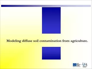
Modeling diffuse soil contamination from agriculture. introduction. SUMMARY: Soil contamination, as defined in the Soil Thematic Strategy. Local soil contamination and Diffuse soil contamination Modeling Tools of Diffuse soil contamination. SWAT Description SWAT application, two cases

E N D
introduction • SUMMARY: • Soil contamination, as defined in the Soil Thematic Strategy. • Local soil contamination and Diffuse soil contamination • Modeling Tools of Diffuse soil contamination. • SWAT Description • SWAT application, two cases • Leaching Modeling. Pesticide soil contamination. • PRZM and PEARL description • PRZM and PEARL application • Conclusion
introduction Soil contamination, as defined in the Soil Thematic Strategy. The introduction of contaminants in the soil may result in damage to or loss of some or several functions of soils and possible cross contamination of water. The occurrence of contaminants in soils above certain levels entails multiple negative consequences for the food chain and thus for human health, and for all types of ecosystems and other natural resources.
Local and Diffuse Soil contamination, Sources. introduction Local Soil contamination, Sources. Local (or point source) contamination is generally associated with mining, industrial facilities, waste landfills and other facilities both in operation and after closure. These activities can pose risks to both soil and water. Diffuse Soil contamination, Sources. Diffuse pollution is generally associated with atmospheric deposition, certain farming practices and inadequate waste and wastewater recycling and treatment.
introduction Diffuse Soil contamination, Sources. • Atmospheric deposition is due to emissions from industry, traffic and agriculture. Deposition of airborne pollutants releases into soils acidifying contaminants (e.g. SO2, NOx), heavy metals (e.g. cadmium, lead arsenic, mercury), and several organic compounds (e.g. dioxins, PCBs, PAHs). • Production systems where a balance between farm inputs and outputs is not achieved in relation to soil and land availability, leads to nutrient imbalances in soil, which frequently result in the contamination of ground- and surface water. • Pesticides are toxic compounds deliberately released into the environment to fight plant pests and diseases. They can accumulate in the soil, leach to the groundwater and evaporate into the air from which further deposition onto soil can take place.They also may affect soil biodiversity and enter the food chain. • With regard to waste, sewage sludge, the final product of the treatment of wastewater, is also raising concern. A whole range of pollutants, such as heavy metals and poorly biodegradable trace organic compounds, potentially contaminates it what can result in an increase of the soil concentrations of these compounds.
introduction Diffuse Soil contamination, Sources. Production systems where a balance between farm inputs and outputs is not achieved in relation to soil and land availability, leads to nutrient imbalances in soil, which frequently result in the contamination of ground- and surface water. Modeling the fate of contaminants requires an understanding of the soil-water-air continuum. The modeling tool should be able to simulated physical, chemical and biological processes occurring in these different compartments.
The modelling approach ... Simulation of soil processes: organic matter turnover, crop growth, nitrogen uptake, water infiltration, evaporation from crop and soil surface, nitrification, denitrification, interception of precipitation and emissions to the atmosphere. AIR Atmospheric deposition Atmospheric emissions N fixation Fertilizer applications Plants consumption Plants consumption Point discharges SOIL Surface and subsurface runoff N Leaching NITRIFICATION/ DENITRIFICATIONSTORAGE RIVER GROUNDWATER
Estimation of loads at representative sites, aggregation at landscape scale, and upscaling to regions . • Calculation of the impacts of the agricultural sector under selected land use scenarios. … a nested approach • Vertical flow in the unsaturated zone links the soil processes to the 2-D overland flow and to the 3-D groundwater flow. • A fully distributed physically based model representing variations in catchment characteristics and driving variables by a network of uniform grids or sub-basins.
An Observational Network of European Watersheds • Scenario analyses (socio-economic, climate, environmental) to improve resource management and provide information that will aid for the sustainable management of the watershed. • Impact assessment of waste management strategies, tourism, urban areas, mining activities, land use changes.
Modeling tools Modeling of Diffuse soil contamination. • Modeling Tools: able to considering processes occurring in the soil-water-air compartments in the studied area, mainly used for Nitrogen and Phosphorus modeling. • SWAT (Soil Water Assessment Tool, Blackland Research Centre, Texas US-Arnold et al., 1992)
SWAT description swat main characteristics basin-scale continuous time daily time step physically based computationally efficient long-term simulations water, sediments, nutrients, pesticides
SWAT description Hydrology model
SWAT Physical model hydrology precipitation surface runoff evapo transpiration lateral flow infiltration
SWAT hydrology Physical model Surface runoff use of SCS curve number method to estimate surface runoff Evapotranspiration Three methods included in SWAT ET is evaluated from soils and plants as well Penman-Monteith Hargreaves Priestley-Taylor Snow melt melting if the second soil layer temperature exceeds 0 C and proportional to the snow pack temperature
SWAT Physical model Soil module Water that enters the soil may move along one of several different pathways. The water may be removed from the soil by plant uptake or evaporation. It can percolate past the bottom of the soil profile and ultimately become aquifer recharge. A final option is that water may move laterally in the profile and contribute to streamflow. Of these different pathways, plant uptake of water removes the majority of water that enters the soil profile. SWAT considers: • Soil Structure • Percolation • Lateral Flow
SWAT hydrology physical model Soil Structure Swat considers three phases in the soil:solid, liquid and gas. The solid phase consists of minerals and/or organic matter that forms the matrix or skeleton.Between the solid particles, soil pores are formed that hold the liquid and gas phases. The soil solution may saturate the soil completely or partially. Swat calculates the balance in every layer and once (..and if ) this layer reach the saturation moves the water to the next one.
SWAT hydrology Percolation physical model percolation Percolation is calculated for each soil layer in the profile. Water is allowed to percolate if the water content exceeds the field capacity water content for that layer. When the soil layer is frozen, no water flow out of the layer is calculated. The volume of water available for percolation in the soil layer is calculated: SW ly excess= FC ly – sSW ly if FC ly > SW ly SW ly excess = 0 , = excess ly if FC ly < or = SW ly where SWly,excess is the drainable volume of water in the soil layer on a given day (mm H2O), SWly is the water content of the soil layer on a given day (mm H2O) and FCly is the water content of the soil layer at field capacity (mm H2O).
SWAT hydrology lateral flow physical model Lateral Flow Lateral flow will be significant in areas with soils having high hydraulic conductivities in surface layers and an impermeable or semipermeable layer at a shallow depth. In such a system, rainfall will percolate vertically until it encounters the impermeable layer. The water then ponds above the impermeable layer forming a saturated zone of water, i.e. a perched water table. This saturated zone is the source of water for lateral subsurface flow.
SWAT weather Physical model driving variables • precipitation daily measurements • temperature • solar radiation • wind speed Monthly measurements • relative humidity In case of missed values, a weather generator is included in the code
Physical model swat sediments sediment yield MUSLE: Modified Universal Soil Loss Equation (USDA, Williams et al. 1977)
Physical model swat crop growth solar radiation energy biomass interception leaf area production index crop heat parameter units crop yield harvest index
Physical model swat nutrients NITROGEN model in SWAT harvest Residue Plant uptake Stable organic N Decay Mineralization Mineralization NO3 Active organic N Denitrification Inorganic fertilizer Organic fertilizer
Physical model swat nutrients PHOSPHORUS model in SWAT Organic fertilizer Mineralization Residue Lumped Active/Stable organic P harvest Mineralization Plant uptake Sediment-bound labile P Dissolved labile P Sediment-bound fixed P Inorganic fertilizer
Models application TWO EXAMPLES DEVELOPED USING SWAT COUPLED WITH GIS (ArcInfo and ArcView, ESRI) OUSE Catchment (UK) BURANA PO di VOLANO Catchment (IT) MAIN ISSUES OF THE MODEL APPLICATIONS Allowing the quantification of the total load of pollutant affecting a watershed. This model should be used to understand how the soil quality and water quantity/quality are affected by agricultural activities.
Examples: OUSE Catchment (UK) Soil Map
Examples: OUSE Catchment (UK) Landuse Map • OUSE Land Use: (%) • FRSE 2.25 • PAST 27.02 • RANGE 32.88 • WWHT 29.10 • URBAN 8.75
OUSE WATERSHED MONTHLY TIME STEP SIMULATION(30 years simulation): FLOW OUT [m3/s] and LINEAR CORRELATION
OUSE WATERSHED MONTHLY TIME STEP SIMULATION(30 years simulation): TOTAL NITROGEN [Kg]
LANDUSE SCENARIO: COMPARISON BETWEEN N EXCESS AND N PLANT UPTAKE WITH TWO DIFFERENT APPLICATION RATE OF ORGANIC NITROGEN IN THE OUSE WATERSHED
LANDUSE SCENARIO: COMPARISON BETWEEN NO3 TO RIVER AND NO3 LEACHING WITH TWO DIFFERENT APPLICATION RATE OF ORGANIC NITROGEN IN THE OUSE WATERSHED 210 Kg/ha ORGANIC NITROGEN AVERAGE ANNUAL CHANGE: -6.34 % 170 Kg/ha ORGANIC NITROGEN
Present scenario Influence of Climate Change on Nitrogen Percolation from Soils to Groundwater Burana-Po di Volano watershed Scenario I GCM Scenario CGCM1 e HadCM2 year 2050 Scenario II NO3 leaching (Kg/ha)
Modeling tools Modeling of Diffuse soil contamination. • Leaching Models: applied to determine the quantity of Pesticide leaching thought the soil profile reaching the shallow aquifer. • PRZM2: Pesticide Root Zone Model, Environmental Protection Agency, US - Carsel et al. 1984. • PEARL: Pesticide Emission Assessment at Regional and Local Scales by Alterra Green World Research.
Models application TWO EXAMPLES DEVELOPED USING PRZM and PEARL coupled with ARCVIEW GIS TREVIGLIO Catchment (IT) EUROPEAN SCALE MAIN ISSUES OF THE MODEL APPLICATIONS Models are run at field and regional scale to be tested (PRZM, PELMO) then the necessary information are collected at European level and run with a model like PEARL (able to work with big database) to estimate the persistence of selected substances at European scale.
Examples: TREVIGLIO catchment (IT) Modeling of Diffuse soil contamination. Regional scale • PRZM2 is a one-dimensional, dynamic, compartmental model that can be used to simulate chemical movement in unsaturated soil systems within and immediately below the plant root zone. It has two major components: • hydrology • chemical transport. • The model was specifically designed to provide loading to selected media, including air, water, groundwater. PRZM2 runs on daily time step. PRZM2 is extensively used from the U.S. Environmental Protection Agency to simulate the transport of field-applied pesticides in the crop root zone.
Examples: TREVIGLIO catchment(IT) Atrazine (app. Rate 1.5 Kg/ha) Alachlor (app. Rate 2.0 Kg/ha)
Use a process based model supported by the FOCUS working group that includes all major processes involved with pesticide transformation and fate. For instance, we are currently using the PEARL model which is used to evaluate the leaching of pesticides to the groundwater in support to the European and Dutch pesticide registration procedures. Bentazone soil concentration 22 and 278 days after application of 0.8 kg/ha of bentazone on field under winter wheat (NL)
Deliverable: map of pesticides persistence in the top layer, in the root zone, and leaching below the root zone Collect the necessary information at European level and run the PEARL model to estimate the persistence of selected substances
CONCLUSION: • These kind of modeling tool could be useful to analyze and simulate the water contamination in a medium-big scale watershed. • They are able to determine soil limitations (topography, rooting depth, chemical fertility, organic carbon) of European soils (using harmonised European soil information system). • It is also possible to derive crop suitability zones and compare the capability maps with land use maps. • Useful to make some general conclusion about the effect of the global climate change could be done. • LIMITATIONS: • The calibration of the model is time-consuming and it would need more efficient tools • The quality of the model simulation depends on the quality of the data available.