Download
1 / 24
240 likes | 315 Vues
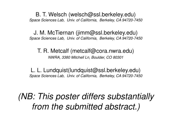
B. T. Welsch (welsch@ssl.berkeley.edu) Space Sciences Lab, Univ. of California, Berkeley, CA 94720-7450 J. M. McTiernan (jimm@ssl.berkeley.edu) Space Sciences Lab, Univ. of California, Berkeley, CA 94720-7450 T. R. Metcalf (metcalf@cora.nwra.edu) NWRA, 3380 Mitchell Ln, Boulder, CO 80301

E N D
B. T. Welsch (welsch@ssl.berkeley.edu)Space Sciences Lab, Univ. of California, Berkeley, CA 94720-7450 J. M. McTiernan (jimm@ssl.berkeley.edu)Space Sciences Lab, Univ. of California, Berkeley, CA 94720-7450 T. R. Metcalf (metcalf@cora.nwra.edu) NWRA, 3380 Mitchell Ln, Boulder, CO 80301 L. L. Lundquist(lundquist@ssl.berkeley.edu)Space Sciences Lab, Univ. of California, Berkeley, CA 94720-7450 (NB: This poster differs substantially from the submitted abstract.)
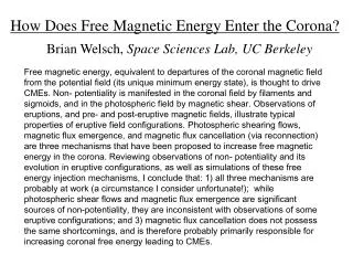
Free magnetic energy is the difference between the energy of a given magnetic field, and the potential magnetic field matching the same normal-field boundary condition. Solar flares and CMEs are thought to be powered by free magnetic energy stored in the coronal field. We apply three methods of calculating changes in the corona’s free magnetic energy to time series of vector magnetograms from NOAA AR 9026, recorded on 25 Jun 2000, around 18:00 UT: • a Modified Magnetic Virial Theorem (MMVT), which uses an integral over the measured field on the photospheric boundary; • Non-linear Force-Free Field (NLFFF) extrapolations, which allow integration of B2/8 over the extrapolation volume; and • the Free-Energy Flux (FEF), which is given by the difference between the energy fluxes into the actual and potential fields. We find: • the MMVT energies are larger than the NLFFF energies, which are, in turn, larger than FEF energy changes; • all calculated energy changes exhibit strong fluctuations, dU (F) ~U(F).
Free energy is the energy difference between the actual and potential field energies. • For a given field B, the magnetic energy is U dV (B·B)/8. • The lowest energy the field could have would match the same boundary condition Bn, but would be current-free (curl-free), or “potential:” B(P) = - , with 2 = 0. Then U(P) dV (B(P) ·B(P) )/8 = dA (· n)/8 • The difference U(F) = U – U (P) is the energy available to power flares and CMEs!
We studied vector magnetogram data from AR 9026, on 05 Jun 2000, near 18:00 UT. • We focussed on IVM magnetograms from c. 17:00 – 19:00 UT. • Average magnetogram cadence was ~ 4 min. • A GOES C3.8 flare occurred near 18:23 UT • 1 Pix ~ 810 km ~ 1.1”
The Magnetic Virial Theorem (MVT) gives field energy via integration over boundary surface. • Unmodified MVT assumes B is force-free, even on the boundaries – but photosphere is forced! • So MVT is usually applied only to chromospheric vector magnetograms, e.g., Metcalf et al., 2003. • Wheatland & Metcalf (2005) proposed a Modified MVT (MMVT), that employs extrapolation to from forced to force-free layer. • Hence, MMVT allows free energy estimation from photospheric magnetograms.
U(F) from MMVT is ~1033erg, with strong fluctuations across the data set.
Non-linear force-free field (NLFFF) extrap-olations give B, allowing integration of B2/8. • Wheatland et al. (2000) described a relaxation method to determine a NLFFF, B(x,y,z), that matches a given magnetic boundary condition. • Specification of B is required on all surfaces: the magnetogram gives the photospheric B(x,y), and B(P) is used on other boundaries. • Strictly, NLFFF extrapolation should not be applied to non-force-free photospheric magnetograms. • McTiernan has implemented this extrapolation procedure in IDL, and distributed it via SSW, in the NLFFF package.
U(F) from NLFFF is ~1032erg, with strong fluctuations across the data set.
The “free energy flux (FEF) density” is the difference between energy fluxes into B and B(P). Depends on photospheric (Bx, By, Bz), (ux,uy), and (Bx(P), By(P)). Requires vector magnetograms. Compute from Bz. What about v or u?
Several techniques exist to determine velocities required to calculate the free energy flux density. • Time series of vector magnetograms can be used with, e.g., ILCT (Welsch et al. 2004), MEF (Longcope 2004), Schuck (2005), and LCT (Démoulin & Berger 2003) to find • Proposed locations of free energy injection can be tested, e.g., • rotating sunspots • shear flows along PILs
We used LCT to derive flows between pairs of boxcar-averaged magnetograms.
The spatially integrated free energy flux could be correlated with flares & CMEs. • Knowledge of the free energy flux density Sz(F) allows computation of total free energy flux, • Large tU(F) could lead to flares/CMEs. • Small flares can dissipate U(F), but should not dissipate much magnetic helicity. • Hence, tracking helicity flux is important, too!
Changes in U(F) derived via FEF are ~1031erg, and vary in both sign and magnitude. Variance estimates were determined by shifting boxcar endpoints.
Cumulative FEF ( U(F)) should match the evolution of U(F) from MMVT & NLFFF. The U(F) plots do not agree.
CONCLUSIONS Using three different methods, we derived estimates for the free magnetic energy present in the coronal magnetic field in AR 9026 near 18:00 UT on 25 Jun 2000: • a Modified Magnetic Virial Theorem (MMVT), which uses an integral over the measured field on the photospheric boundary; • Non-linear Force-Free Field (NLFFF) extrapolations, which allow integration of B2/8 over the extrapolation volume; and • the Free-Energy Flux (FEF), which is given by the difference between the energy fluxes into the actual and potential fields. We find: • the MMVT energies are larger than the NLFFF energies, which are, in turn, larger than FEF energy changes; • the MMVT, NLFFF, and FEF energies are not correlated in time; • all calculated energy changes exhibit strong fluctuations, dU (F) ~U(F).
References • Démoulin & Berger, 2003: Magnetic Energy and Helicity Fluxes at the Photospheric Level, Démoulin, P., and Berger, M. A. Sol. Phys., v. 215, # 2, p. 203-215. • Longcope, 2004:Inferring a Photospheric Velocity Field from a Sequence of Vector Magnetograms: The Minimum Energy Fit, ApJ, v. 612, # 2, p. 1181-1192. • Metcalf et al., 2005:Magnetic Free Energy in NOAA Active Region 10486 on 2003 October 29, Metcalf, T. R., Leka, K. D., Mickey, D. L., ApJ, 623, # 1, pp. L53-L56. • Metcalf et al., 1995:Is the solar chromospheric magnetic field force-free? Metcalf, T. R., Jiao, L., McClymont, A. N., Canfield, R. C., Uitenbroek, H. , ApJ, v. 439, #1, p. 474- 481. • Schuck, 2005:Tracking Magnetic Footpoints with the Magnetic Induction Equation, ApJ (submitted, 2005) • Welsch et al., 2004:ILCT: Recovering Photospheric Velocities from Magnetograms by Combining the Induction Equation with Local Correlation Tracking, Welsch, B. T., Fisher, G. H., Abbett, W.P., and Regnier, S., ApJ, v. 610, #2, p. 1148-1156. • Welsch, 2005:Magnetic Flux Cancellation and Coronal Magnetic Energy, ApJ, in press. • Wheatland et al., 2000:An Optimization Approach to Reconstructing Force-free Fields, Wheatland, M. S., Sturrock, P. A., Roumeliotis, ApJ, v. 540, #2, p. 1150-1155. • Wheatland & Metcalf, 2005:An improved virial estimate of solar active region energy, Wheatland, M.S. and Metcalf, T.R. , ApJ, in press. (v. 636, #2, 10 Jan. 2006) [on astro-ph]
In ideal MHD, photospheric flows move mag-netic flux with a flux transport rate, Bnuf. (3) Demoulin & Berger (2003): Apparent motion of flux on a surface can arise from horizontal and/or vertical flows. In either case, uf represents “flux transport velocity.”
Magnetic diffusivity also causes flux transport, as field lines can slip through the plasma. • Non-ideal processes are truly 3D effects, but can be approximated as 2D diffusion. • Hence, approximate non-ideal flux transport term in Fick’s Law form,
The change in the actual magnetic energy is given by the Poynting flux, c(E x B)/4. • In ideal MHD, E = -(v x B)/c, so: • uf is the flux transport velocity; uf B (see eqn. [3]) • uf is related to induction eqn’s z-component, (1)
A “Poynting-like” flux can be derived for the potential magnetic field, B(P), too. • B evolves via the induction equation, meaning (ideally) its topology is conserved. • B(P) does not necessarily obey the induction equation, meaning its topology can change! • But energy change is Poynting-like: from equations (1) (2)!
Also works w/ non-ideal terms… at eqn’s left is valid w/any non-ideal term!