Solving Polynomial Systems by Homotopy Continuation

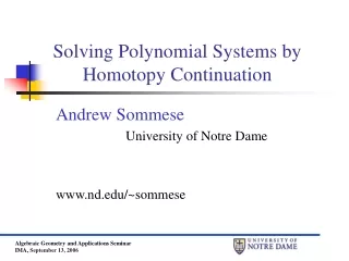
Solving Polynomial Systems by Homotopy Continuation Andrew Sommese University of Notre Dame www.nd.edu/~sommese

Reference on the area up to 2005: • A.J. Sommese and C.W. Wampler, Numerical solution of systems of polynomials arising in engineering and science, (2005), World Scientific Press. • Survey covering other topics • T.Y. Li, Numerical solution of polynomial systems by homotopy continuation methods, in Handbook of Numerical Analysis, Volume XI, 209-304, North-Holland, 2003.

Overview • Solving Polynomial Systems • Computing Isolated Solutions • Homotopy Continuation • Case Study: Alt’s nine-point path synthesis problem for planar four-bars • Positive Dimensional Solution Sets • How to represent them • Decomposing them into irreducible components • Numerical issues posed by multiplicity greater than one components • Deflation and Endgames • Bertini and the need for adaptive precision • A Motivating Problem and an Approach to It • Fiber Products • A positive dimensional approach to finding isolated solutions equation-by-equation

Solving Polynomial Systems • Find all solutions of a polynomial system on :

Why? • To solve problems from engineering and science.

Characteristics of Engineering Systems • systems are sparse: they often have symmetries and have much smaller solution sets than would be expected.

Characteristics of Engineering Systems • systems are sparse: they often have symmetries and have much smaller solution sets than would be expected. • systems depend on parameters: typically they need to be solved many times for different values of the parameters.

Characteristics of Engineering Systems • systems are sparse: they often have symmetries and have much smaller solution sets than would be expected. • systems depend on parameters: typically they need to be solved many times for different values of the parameters. • usually only real solutions are interesting

Characteristics of Engineering Systems • systems are sparse: they often have symmetries and have much smaller solution sets than would be expected. • systems depend on parameters: typically they need to be solved many times for different values of the parameters. • usually only real solutions are interesting. • usually only finite solutions are interesting.

Characteristics of Engineering Systems • systems are sparse: they often have symmetries and have much smaller solution sets than would be expected. • systems depend on parameters: typically they need to be solved many times for different values of the parameters. • usually only real solutions are interesting. • usually only finite solutions are interesting. • nonsingular isolated solutions were the center of attention.

Computing Isolated Solutions • Find all isolated solutions in of a system on n polynomials:

Solving a system • Homotopy continuation is our main tool: • Start with known solutions of a known start system and then track those solutions as we deform the start system into the system that we wish to solve.

Path Tracking This method takes a system g(x) = 0, whose solutions we know, and makes use of a homotopy, e.g., Hopefully, H(x,t) defines “nice paths” x(t) as t runs from 1 to 0. They start at known solutions of g(x) = 0 and end at the solutions of f(x) at t = 0.

The paths satisfy the Davidenko equation • To compute the paths: use ODE methods to predict and Newton’s method to correct.

x1(t) x2(t) x3(t) x4(t) Known solutions of g(x)=0 Solutions of f(x)=0 t=0 H(x,t) = (1-t) f(x) + t g(x) t=1

x* { xj(t) 0 Dt prediction Newton correction 1

Algorithms • middle 80’s: Projective space was beginning to be used, but the methods were a combination of differential topology and numerical analysis with homotopies tracked exclusively through real parameters. • early 90’s: algebraic geometric methods worked into the theory: great increase in security, efficiency, and speed.

Uses of algebraic geometry Simple but extremely useful consequence of algebraicity [A. Morgan (GM R. & D.) and S.] • Instead of the homotopy H(x,t) = (1-t)f(x) + tg(x) use H(x,t) = (1-t)f(x) + gtg(x)

Genericity • Morgan + S. : if the parameter space is irreducible, solving the system at a random point simplifies subsequent solves: in practice speedups by factors of 100.

Endgames (Morgan, Wampler, and S.) • Example: (x – 1)2 - t = 0 We can uniformize around a solution at t = 0. Letting t = s2, knowing the solution at t = 0.01, we can track around |s| = 0.1 and use Cauchy’s Integral Theorem to compute x at s = 0.

Special Homotopies to take advantage of sparseness

Multiprecision • Not practical in the early 90’s! • Highly nontrivial to design and dependent on hardware • Hardware too slow

Hardware • Continuation is computationally intensive. On average: • in 1985: 3 minutes/path on largest mainframes.

Hardware • Continuation is computationally intensive. On average: • in 1985: 3 minutes/path on largest mainframes. • in 1991: over 8 seconds/path, on an IBM 3081; 2.5 seconds/path on a top-of-the-line IBM 3090.

Hardware • Continuation is computationally intensive. On average: • in 1985: 3 minutes/path on largest mainframes. • in 1991: over 8 seconds/path, on an IBM 3081; 2.5 seconds/path on a top-of-the-line IBM 3090. • 2006: about 10 paths a second on a single processor desktop CPU; 1000’s of paths/second on moderately sized clusters.

A Guiding Principle then and now • Algorithms must be structured – when possible – to avoid extra paths and especially those paths leading to singular solutions: find a way to never follow the paths in the first place.

Continuation’s Core Computation • Given a system f(x) = 0 of n polynomials in n unknowns, continuation computes a finite set S of solutions such that: • any isolated root of f(x) = 0 is contained in S; • any isolated root “occurs” a number of times equal to its multiplicity as a solution of f(x) = 0; • S is often larger than the set of isolated solutions.

Case Study: Alt’s Problem • We follow

A four-bar planar linkage is a planar quadrilateral with a rotational joint at each vertex. • They are useful for converting one type of motion to another. • They occur everywhere.

How Do Mechanical Engineers Find Mechanisms? • Pick a few points in the plane (called precision points) • Find a coupler curve going through those points • If unsuitable, start over.

Having more choices makes the process faster. • By counting constants, there will be no coupler curves going through more than nine points.

Nine Point Path-Synthesis Problem H. Alt, Zeitschrift für angewandte Mathematik und Mechanik, 1923: • Given nine points in the plane, find the set of all four-bar linkages, whose coupler curves pass through all these points.

First major attack in 1963 by Freudenstein and Roth.

P0 δj Pj y x C D D′ µj λj u v b C′

P0 δj Pj θj y yeiθj C b b-δj µj v v = y – b veiμj = yeiθj - (b - δj) = yeiθj + δj - b C′

We use complex numbers (as is standard in this area) Summing over vectors we have 16 equations plus their 16 conjugates

This gives 8 sets of 4 equations: in the variables a, b, x, y, and for j from 1 to 8.

Multiplying each side by its complex conjugate and letting we get 8 sets of 3 equations in the 24 variables with j from 1 to 8.

in the 24 variables with j from 1 to 8.

Using Cramer’s rule and substitution we have what is essentially the Freudenstein-Roth system consisting of 8 equations of degree 7. Impractical to solve in early 90’s: 78 = 5,764,801solutions.

Newton’s method doesn’t find many solutions: Freudenstein and Roth used a simple form of continuation combined with heuristics. • Tsai and Lu using methods introduced by Li, Sauer, and Yorke found only a small fraction of the solutions. That method requires starting from scratch each time the problem is solved for different parameter values

Solve by Continuation All 2-homog. systems All 9-point systems “numerical reduction” to test case (done 1 time) synthesis program (many times)

Intermission

Positive Dimensional Solution Sets We now turn to finding the positive dimensional solution sets of a system

How to represent positive dimensional components? • S. + Wampler in ’95: • Use the intersection of a component with generic linear space of complementary dimension. • By using continuation and deforming the linear space, as many points as are desired can be chosen on a component.

Use a generic flag of affine linear spaces to get witness point supersets This approach has 19th century roots in algebraic geometry

Solving Polynomial Systems by Homotopy Continuation