Ad Hoc Networks
Ad Hoc Networks. Dirk Grunwald University of Colorado, Boulder. Outline. Review of routing in wired networked Routing domains & levels RIP routing Distance Vector Routing Examples of RIP information & management OSPF routing Link state routing Routing in ad-hoc wireless networks.

Ad Hoc Networks
E N D
Presentation Transcript
Ad Hoc Networks Dirk GrunwaldUniversity of Colorado, Boulder
Outline • Review of routing in wired networked • Routing domains & levels • RIP routing • Distance Vector Routing • Examples of RIP information & management • OSPF routing • Link state routing • Routing in ad-hoc wireless networks
Gateway Hierarchy InternetCore AutonomousSystem(AS) AutonomousSystem(AS)
Two levels of Routing Protocols RoutingDomain RoutingDomain IGP IGP EGP RoutingDomain EGP EGP Intra-domainrouting protocol Exteriorrouting protocol IGP
Routing Protocols • Intra-domain Gateway Protocols • RIP • RIP V2 • OSPF - open shortest path first • IS-IS (similar to OSPF) • Exterior Gateway Protocols • EGP • BGP
RIP • Distance vector routing algorithm based on hops that communicates between routers using UDP • On initialization, router determines all available interfaces and sends a ROUTE REQUEST packet out each interface. Special request for “send everything” • On receipt of request, • Either return everything • Or, for each requested destination, return distance to that destination + 1 • On response • Update routing tables
RIP V1 Protocol Command Version MBZ Address Family MBZ 32-bit IP address MBZ MBZ Metric (value of 1..16) Up to 24 more routes in same format...
Metrics N2 is 1 hop N1 Route to N3via R2 withhop count of 2 R1 N3 is 1 hop N2 N1 is 1 hop R2 N3 N2 is 1 hop
Problems • Hop count limited to 15 • Can only be used within an AS where maximum network diameter of 15 • It’s based on HOPS, not e.g., latency or bandwidth • No notion of subnet addressing in RIP V1
RIP V2 Protocol Command Version Routing domain Address Family Route tag 32-bit IP address 32-bit subnet mask 32-bit next-hop IP address Metric (value of 1..16) Up to 24 more routes in same format...
RIP V2 • Routing domain is an identifier of the routing daemon • Process ID in UNIX • …So you can run multiple instances of RIP • Route tag carries an autonomous system number for EGP and BGP • Next op address is where packets corresponding to that (sub)network should be sent. A value of zero means send to the system sending RIP info. • Simple authentication scheme with clear-text password
Distance Vector Routing • Also called Bellman-Ford or Ford-Fulkerson algorithms • Used by RIP • Each router is responsible for keeping track of and informing its neighbors of its distance to each destination • The router computes its distance to a destination based on its neighbors distance to the destination • Router must know it’s own ID and the cost of its links to each neighbor
Distance Vector Routing For Address “D” 17 2 Link number 1 2 35 R 3 5 4 41 5 Link cost
Distance Vector Routing For Address “D” 97 81 17 2 Cost from neighbor to destination D 1 2 35 R 62 3 5 4 41 5 29 118
Distance Vector Routing For Address “D” 97 81 99 17 2 Cost for Rto get to Dvia this link 98 1 2 35 R 62 3 5 97 4 41 5 70 123 29 118 Minimumcost route
Distance Vector Routing For Address “D” 70 70 17 2 Cost fromR to D 1 2 35 R 70 3 5 4 41 5 70 70
Problems With Distance Vector • Slow convergence to the lowest cost route • Slow recovery time if there are link failures • Slow recovery leads to routing problems during recovery • Router loops • Count to infinity
2 4 3 2 1 2 3 1 Count To Infinity (worse case loop) A A A A B B B B C
OSPF - Open Shortest Path First • OSPF uses IP directly (I.e., like ICMP) • Routes calculated based on Type of Service (TOS) • Each interface is assigned a dimensionless cost,for each TOS • If several equal-cost routes are available,traffic is load-balanced • Subnets are associated with each advertised route • Supports authentication • Uses multicast to distribute information
Link State Routing • Used by OSPF and IS-IS • Construct a Link State Packet (LSP) that lists neighbors and costs to get to those neighbors • LSP = (destination, path cost, forwarding direction) • Use Dijkstra’s algorithm to compute global routes as a tree from the current router
Dijkstra’s Algorithm • Two sets of paths: PATH and TENT(ative) • LSP = (destination, path cost, forwarding direction) (1) Place (self, 0,0) in path (2) For any (D,C,F) placed in PATH, examine D’s LSP. For each Neighbor of D listed in D’s LSP with a link cost to N of c, see if (N, c, …) is already in TENT or PATH. If not listed, or if c is less than existing cost, add (N, C+c,…) to TENT (3) Terminate if TENT is empty, otherwise find (D,C,F) with minimum C and add that to PATH. Goto (2)
Example of Dijkstra’s Algorithm C(0) Cost F(2) B(2) G(5) Destination
Example of Dijkstra’s Algorithm C(0) F(2) B(2) G(5) E(6) G(3) Since B and F have samecost, select one at random.Place “F” in PATH. Cost relative to node C
Example of Dijkstra’s Algorithm C(0) F(2) B(2) G(5) E(6) Better pathto G exists G(3)
Example of Dijkstra’s Algorithm Add B to Path C(0) F(2) B(2) A(8) E(3) E(6) G(3)
Example of Dijkstra’s Algorithm C(0) F(2) B(2) A(8) E(3) E(6) G(3) Better pathto E exists
Example of Dijkstra’s Algorithm C(0) Add E to path F(2) B(2) A(8) E(3) G(3) D(5)
Original Distribution of LSP’s • Neighbor-to-neighbor protocol for LSP distribution • Each LSP consists of • Identity of router generating the LSP • A sequence number • The time left until the LSP should be discarded • A list of neighbors, and the cost of links to each • LSP is broadcast to all neighbors • LSP’s have a 64 second lifetime - each router must resend each minute • Wrap-around comparison on sequence numbers used
Problem in 1991 • A router announced LSP’s with random TTL’s • a < b < c <a • Each router that processed one of these LSP’s over-wrote the one in memory and generated more copies of the bad LSP, since it thought that this LSP was newer & needed to be propagated to neighbors • The TTL field never changed because of the rapid rate of updates
Revised method using 32-bit sequences • LSP’s compared only by their sequence numbers - if you get LSP with sequence S & T, and S < T, then T is more recent (no matter what TTL says) • LSP’s are purged when old, based on TTL. Every router decrements TTL • When TTL reaches 0, router refloods the LSP. Given (sequence, TTL) (S,x) & (T,y) then S < T if x = 0, but not otherwise • LSP’s generated much less frequently (~1hr) • Router starts with the lowest sequence number. If the network retains old LSP, it will be flooded back to source, which then knows “current” sequence number to use
A Simple Ad-Hoc Network D. Johnson and D. Maltz A can not communicate directly with C
Applications of Ad Hoc Networks • Useful for forming instant networks, without administration and reduced set-up cost. • Conferences / meetings / lectures – shared notes, whiteboard, file sharing, etc • Emergency Services / Search & Rescue – location, situation information, status & messaging • People may move between an infrastructure network and an adhoc network • May be important for vehicles – cars could form an “adhoc” network while on the move
Challenges & Future Research Areas • Multicast • QoS support • “plain” and “adaptive” QoS • Power-aware Routing • Location-Aided Routing • Media Access Control • Security • Service Discovery
Table Driven Methods • Attempt to maintain consistent, up-to-date routing information from each node to every other node in the network • Perfect for “connectionless” traffic where you may send traffic to any node at any time • Respond to changes by propagating updates throughout the network to maintain a consistent network view.
Source Initiated Methods • Routes are only created when desired by the source node • When a node requires a route, it initiates a “route discovery process”. • The route discovery finishes either when a route is discovered or all possible communication paths have been examined. • Once a route is established, is it maintained by some sort of route maintenance protocol
DSDV – Destination Sequenced Distance Vector Routing • Based on Bellman-Ford routing mechanism • Each node maintains routing table that records all possible destinations and the number of hops to those destinations • Each entry is marked with a sequence number assigned by the destination node. These sequence numbers are used to distinguish “old” vs “new” routes. • Routing tables are periodically transmitted to maintain table consistency • A “full dump” record reports on the entire routing table. Lots of traffic, since each table is probably larger than the network protocol data unit. • Incremental updates provide information since last “full dump”
DSDV • A new route broadcasts contain • The address of the destination • The number of hops to reach the destination • The sequence number of the information • Sequence number unique to this broadcast • Route labeled with most recent sequence number is always used • If two event have the same sequence number, the route with the smaller metric (== shorter route) is used • Hosts also keep track of the the settling time of routes, or the weighted average time that routes to a destination will fluctuate before the route with the best metric is received
Clusterhead Gateway Switch Routing (CGSR) • Clustered multi-hop routing protocol • Node routes to “cluster head” • Clusterhead routes to other “cluster-head” by gateways • Eventually, clusterhead routes to specific node Gateway 5 ClusterHead 3 4 6 1 8 2 7
CGSR • Clusters allow channel & bandwidth allocation • Nodes only speak to cluster heads • Gateways speak to one or more cluster heads • Cluster election algorithm picks cluster head • A “least cluster change” algorithm is used to reduce the election overhead • Re-election only occurs when two cluster heads move within communication range or a node is “lost” by moving out of communication range. • DSDV used as the underlying scheme
CGSR Example 5 3 4 7 1 9 6 2 8
CGSR • Each node must keep a “cluster member table” where it stores destination cluster head for each mobile node • Can that really be true? Shouldn’t the cluster head be the only one that needs to maintain this? • Cluster tables are broadcast using DSDV algorithm • Each node also maintains a routing table, which is used to specify the next hop towards the destination • To route, the node looks in the cluster table to determine the nearest cluster head and then uses routing table to determine how to reach that cluster head. • Makes no sense.
Wireless Routing Protocol • Each node maintains • Distance Table • Routing Table • Link-Cost Table • Message Retransmission List • Updates are exchanged with neighbor nodes • Destination, distance to destination, predecessor of the destination (next hop) • Messages are sent when a link status changes or after updates from their neighbors • Nodes learn of the existence of their neighbors from the receipt of ACKs
Ad-Hoc On Demand Distance Vector (AODV) • Based on DSDV, but builds routes on demand. • If node S has a message for D, but no route, it starts a path discovery process. • Broadcasts / floods a Route Request (RREQ) • Eventually, either the destination (D) or an intermediate node with a “fresh enough” route cache is reached. • Each node maintains a sequence number as well as a broadcast ID • Broadcast ID is incremented for each RREQ • Combination of node address & broadcast ID uniquelyidentifies a RREQ
AODV • The source RREQ also includes the most recent sequence number for the destination • Intermediate nodes can only respond if they have “fresher” information -- prevents replying with stale information • Once the message reaches the destination (or intermediary), a Route Reply (RREP) is sent back along the path by which each node first received a route request • Nodes in that route establish forward routes for the destination • Only supports symmetric links!
AODV • If a source node moves, it can re-initiate the route discovery protocol to find a new route • If a node along the route moves, upstream neighbors notice and propogate a “link failure notification” message to each upstream neighbor. • This is propagated “until the source node is reached” • How is this known? Must be imprecise statement • “Hello” messages are used to maintain local connectivity
Dynamic Source Routing • The source specifies entire route • Assumes the network is fairly small • But, no periodic routing advertisements • Uses a source route cache • Route discovery protocol uses a route request message containing • Destination address • Source address • Unique ID • Each node receiving a RREQ checks to see if it knows of a route to the destination. If note, it adds its own address to the Route Record and then forwards the packet on out-going links.