Uniprocessor Optimizations and Matrix Multiplication

1. Uniprocessor Optimizations and Matrix Multiplication

2. Outline • Parallelism in Modern Processors • Memory Hierarchies • Matrix Multiply Cache Optimizations

3. Idealized Uniprocessor Model • Processor names bytes, words, etc. in its address space • These represent integers, floats, pointers, arrays, etc. • Exist in the program stack, static region, or heap • Operations include • Read and write (given an address/pointer) • Arithmetic and other logical operations • Order specified by program • Read returns the most recently written data • Compiler and architecture translate high level expressions into “obvious” lower level instructions • Hardware executes instructions in order specified by compiler • Cost • Each operations has roughly the same cost (read, write, add, multiply, etc.)

4. Uniprocessors in the Real World • Real processors have • registers and caches • small amounts of fast memory • store values of recently used or nearby data • different memory ops can have very different costs • parallelism • multiple “functional units” that can run in parallel • different orders, instruction mixes have different costs • pipelining • a form of parallelism, like an assembly line in a factory • Why is this your problem? In theory, compilers understand all of this and can optimize your program; in practice they don’t.

5. 30 40 40 40 40 20 A B C D What is Pipelining? Dave Patterson’s Laundry example: 4 people doing laundry wash (30 min) + dry (40 min) + fold (20 min) • In this example: • Sequential execution takes 4 * 90min = 6 hours • Pipelined execution takes 30+4*40+20 = 3.3 hours • Pipelining helps throughput, but not latency • Pipeline rate limited by slowest pipeline stage • Potential speedup = Number pipe stages • Time to “fill” pipeline and time to “drain” it reduces speedup 6 PM 7 8 9 Time T a s k O r d e r

6. Limits to Instruction Level Parallelism (ILP) • Limits to pipelining: Hazards prevent next instruction from executing during its designated clock cycle • Structural hazards: HW cannot support this combination of instructions (single person to fold and put clothes away) • Data hazards: Instruction depends on result of prior instruction still in the pipeline (missing sock) • Control hazards: Caused by delay between the fetching of instructions and decisions about changes in control flow (branches and jumps). • The hardware and compiler will try to reduce these: • Reordering instructions, multiple issue, dynamic branch prediction, speculative execution… • You can also enable parallelism by careful coding

7. Outline • Parallelism in Modern Processors • Memory Hierarchies • Matrix Multiply Cache Optimizations

8. Memory Hierarchy • Most programs have a high degree of locality in their accesses • spatial locality: accessing things nearby previous accesses • temporal locality: reusing an item that was previously accessed • Memory hierarchy tries to exploit locality processor control Second level cache (SRAM) Secondary storage (Disk) Main memory (DRAM) Tertiary storage (Disk/Tape) datapath on-chip cache registers Speed (ns): 1 10 100 10 ms 10 sec Size (bytes): 100s Ks Ms Gs Ts

9. Processor-DRAM Gap (latency) • Memory hierarchies are getting deeper • Processors get faster more quickly than memory µProc 60%/yr. 1000 CPU “Moore’s Law” 100 Processor-Memory Performance Gap:(grows 50% / year) Performance 10 DRAM 7%/yr. DRAM 1 1980 1981 1982 1983 1984 1985 1986 1987 1988 1989 1990 1991 1992 1993 1994 1995 1996 1997 1998 1999 2000 Time

10. Experimental Study of Memory • Microbenchmark for memory system performance • time the following program for each size(A) and stride s • (repeat to obtain confidence and mitigate timer resolution) • for array A of size from 4KB to 8MB by 2x • for stride s from 8 Bytes (1 word) to size(A)/2 by 2x • for i from 0 to size by s • load A[i] from memory (8 Bytes)

11. Memory Hierarchy on a Sun Ultra-IIi Sun Ultra-IIi, 333 MHz Array size Mem: 396 ns (132 cycles) L2: 2 MB, 36 ns (12 cycles) L1: 16K, 6 ns (2 cycle) L1: 16 byte line L2: 64 byte line 8 K pages See www.cs.berkeley.edu/~yelick/arvindk/t3d-isca95.ps for details

12. Memory Hierarchy on a Pentium III Array size Katmai processor on Millennium, 550 MHz L2: 512 KB 60 ns L1: 64K 5 ns, 4-way? L1: 32 byte line ?

13. Lessons • Actual performance of a simple program can be a complicated function of the architecture • Slight changes in the architecture or program change the performance significantly • To write fast programs, need to consider architecture • We would like simple models to help us design efficient algorithms • Is this possible? • We will illustrate with a common technique for improving cache performance, called blocking or tiling • Idea: used divide-and-conquer to define a problem that fits in register/L1-cache/L2-cache

14. Outline • Parallelism in Modern Processors • Memory Hierarchies • Matrix Multiply Cache Optimizations

15. Note on Matrix Storage • A matrix is a 2-D array of elements, but memory addresses are “1-D” • Conventions for matrix layout • by column, or “column major” (Fortran default) • by row, or “row major” (C default) Row major Column major 0 5 10 15 0 1 2 3 1 6 11 16 4 5 6 7 2 7 12 17 8 9 10 11 3 8 13 18 12 13 14 15 4 9 14 19 16 17 18 19

16. Optimizing Matrix Addition for Caches • Dimension A(n,n), B(n,n), C(n,n) • A, B, C stored by column (as in Fortran) • Algorithm 1: • for i=1:n, for j=1:n, A(i,j) = B(i,j) + C(i,j) • Algorithm 2: • for j=1:n, for i=1:n, A(i,j) = B(i,j) + C(i,j) • What is “memory access pattern” for Algs 1 and 2? • Which is faster? • What if A, B, C stored by row (as in C)?

17. Key to algorithm efficiency Key to machine efficiency Using a Simple Model of Memory to Optimize • Assume just 2 levels in the hierarchy, fast and slow • All data initially in slow memory • m = number of memory elements (words) moved between fast and slow memory • tm = time per slow memory operation • f = number of arithmetic operations • tf = time per arithmetic operation << tm • q = f / m average number of flops per slow element access • Minimum possible time = f* tf when all data in fast memory • Actual time • Larger q means Time closer to minimum f * tf f * tf + m * tm = f * tf * (1 + tm/tf * 1/q)

18. Simple example using memory model • To see results of changing q, consider simple computation • Assume tf=1 Mflop/s on fast memory • Assume moving data is tm = 10 • Assume h takes q flops • Assume array X is in slow memory s = 0 for i = 1, n s = s + h(X[i]) • So m = n and f = q*n • Time = read X + compute = 10*n + q*n • Mflop/s = f/t = q/(10 + q) • As q increases, this approaches the “peak” speed of 1 Mflop/s

19. Warm up: Matrix-vector multiplication {implements y = y + A*x} for i = 1:n for j = 1:n y(i) = y(i) + A(i,j)*x(j) A(i,:) + = * y(i) y(i) x(:)

20. Warm up: Matrix-vector multiplication {read x(1:n) into fast memory} {read y(1:n) into fast memory} for i = 1:n {read row i of A into fast memory} for j = 1:n y(i) = y(i) + A(i,j)*x(j) {write y(1:n) back to slow memory} • m = number of slow memory refs = 3n + n2 • f = number of arithmetic operations = 2n2 • q = f / m ~= 2 • Matrix-vector multiplication limited by slow memory speed

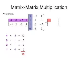
21. “Naïve” Matrix Multiply {implements C = C + A*B} for i = 1 to n for j = 1 to n for k = 1 to n C(i,j) = C(i,j) + A(i,k) * B(k,j) A(i,:) C(i,j) C(i,j) B(:,j) = + *

22. “Naïve” Matrix Multiply {implements C = C + A*B} for i = 1 to n {read row i of A into fast memory} for j = 1 to n {read C(i,j) into fast memory} {read column j of B into fast memory} for k = 1 to n C(i,j) = C(i,j) + A(i,k) * B(k,j) {write C(i,j) back to slow memory} A(i,:) C(i,j) C(i,j) B(:,j) = + *

23. “Naïve” Matrix Multiply Number of slow memory references on unblocked matrix multiply m = n3 read each column of B n times + n2 read each row of A once + 2n2 read and write each element of C once = n3 + 3n2 So q = f / m = 2n3 / (n3 + 3n2) ~= 2 for large n, no improvement over matrix-vector multiply A(i,:) C(i,j) C(i,j) B(:,j) = + *

24. Blocked (Tiled) Matrix Multiply Consider A,B,C to be N by N matrices of b by b subblocks where b=n / N is called the block size for i = 1 to N for j = 1 to N {read block C(i,j) into fast memory} for k = 1 to N {read block A(i,k) into fast memory} {read block B(k,j) into fast memory} C(i,j) = C(i,j) + A(i,k) * B(k,j) {do a matrix multiply on blocks} {write block C(i,j) back to slow memory} A(i,k) C(i,j) C(i,j) = + * B(k,j)

25. Blocked (Tiled) Matrix Multiply Recall: m is amount memory traffic between slow and fast memory matrix has nxn elements, and NxN blocks each of size bxb f is number of floating point operations, 2n3 for this problem q = f / m is our measure of algorithm efficiency in the memory system So: m = N*n2 read each block of B N3 times (N3 * n/N * n/N) + N*n2 read each block of A N3 times + 2n2 read and write each block of C once = (2N + 2) * n2 So q = f / m = 2n3 / ((2N + 2) * n2) ~= n / N = b for large n So we can improve performance by increasing the blocksize b Can be much faster than matrix-vector multiply (q=2)

26. Limits to Optimizing Matrix Multiply The blocked algorithm has ratio q ~= b • The large the block size, the more efficient our algorithm will be • Limit: All three blocks from A,B,C must fit in fast memory (cache), so we cannot make these blocks arbitrarily large: 3b2 <= M, so q ~= b <= sqrt(M/3) There is a lower bound result that says we cannot do any better than this (using only algebraic associativity) Theorem (Hong & Kung, 1981): Any reorganization of this algorithm (that uses only algebraic associativity) is limited to q = O(sqrt(M))

27. Basic Linear Algebra Subroutines • Industry standard interface (evolving) • Vendors, others supply optimized implementations • History • BLAS1 (1970s): • vector operations: dot product, saxpy (y=a*x+y), etc • m=2*n, f=2*n, q ~1 or less • BLAS2 (mid 1980s) • matrix-vector operations: matrix vector multiply, etc • m=n^2, f=2*n^2, q~2, less overhead • somewhat faster than BLAS1 • BLAS3 (late 1980s) • matrix-matrix operations: matrix matrix multiply, etc • m >= 4n^2, f=O(n^3), so q can possibly be as large as n, so BLAS3 is potentially much faster than BLAS2 • Good algorithms used BLAS3 when possible (LAPACK) • Seewww.netlib.org/blas, www.netlib.org/lapack

28. BLAS speeds on an IBM RS6000/590 Peak speed = 266 Mflops Peak BLAS 3 BLAS 2 BLAS 1 BLAS 3 (n-by-n matrix matrix multiply) vs BLAS 2 (n-by-n matrix vector multiply) vs BLAS 1 (saxpy of n vectors)

29. Locality in Other Algorithms • The performance of any algorithm is limited by q • In matrix multiply, we increase q by changing computation order • increased temporal locality • For other algorithms and data structures, even hand-transformations are still an open problem • sparse matrices (reordering, blocking) • trees (B-Trees are for the disk level of the hierarchy) • linked lists (some work done here)

30. Optimizing in Practice • Tiling for registers • loop unrolling, use of named “register” variables • Tiling for multiple levels of cache • Exploiting fine-grained parallelism in processor • superscalar; pipelining • Complicated compiler interactions • Automatic optimization an active research area • BeBOP: www.cs.berkeley.edu/~richie/bebop • PHiPAC: www.icsi.berkeley.edu/~bilmes/phipac in particular tr-98-035.ps.gz • ATLAS: www.netlib.org/atlas

31. Summary • Performance programming on uniprocessors requires • understanding of fine-grained parallelism in processor • produce good instruction mix • understanding of memory system • levels, costs, sizes • improve locality • Blocking (tiling) is a basic approach • Techniques apply generally, but the details (e.g., block size) are architecture dependent • Similar techniques are possible on other data structures and algorithms