websites
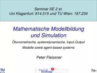
Seminar SE 2 st. Uni Klagenfurt: 814.515 und Uni Wien: 562.430 Mathematische Modellbildung und Simulation Ökonometrische, systemdynamische, Input-Output Modelle sowie agent-based systems Peter Fleissner Institut für Gestaltungs- und Wirkungsforschung. websites. Allgemeines

websites
E N D
Presentation Transcript
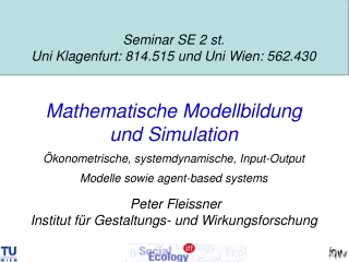
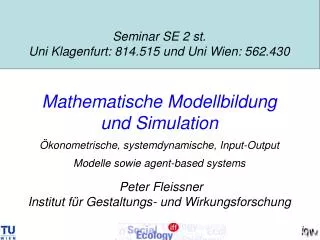
Seminar SE 2 st.Uni Klagenfurt: 814.515 und Uni Wien: 562.430Mathematische Modellbildung und SimulationÖkonometrische, systemdynamische, Input-Output Modelle sowie agent-based systemsPeter FleissnerInstitut für Gestaltungs- und Wirkungsforschung
websites Allgemeines • http://www.iff.ac.at/socec/lehre/lehre_aktuell.php Laufende Ereignisse, Skripten, Termine • http://cartoon.iguw.tuwien.ac.at/zope/lvas/MathMod
Termine • Vorbespr: Donnerstag; 3. März 2005, 17 Uhr • 1. Block: Montag, 7. März (9 -17 Uhr) • 2. Block: Donnerstag, 17. März (9 Uhr) • Vortrag ANYLOGIC TEAM (Ort: Kontaktraum der TU, Gusshausstrasse 25-29, 6. Stock) • 3. Block: Montag, 4. April (9 -17 Uhr) • 4. Block: Montag, 11. April (9 -17 Uhr) • 5. Block: Montag, 2. Mai (9 -17 Uhr) • Ab 15:30 Uhr: Vortrag DI Klug, Seibersdorf • Die ganztägigen Termine finden im Seminarraum 187-2 bzw. im Computerlabor des IGW statt
Ausblick Teil 5 (Montag, 2. Mai, ganzer Tag) • Agent-based modelling • Praktische Beispiele, Vortrag DI Klug ab 15:30 Uhr
Teil 4 Montag, 11. April, ganzer Tag • Volkswirtschaftliche Gesamtrechung (Einführung) • Grundzüge der Input-Output-Analyse, • Mehrebenenökonomie • Anwendungen auf volkswirtschaftliche Modelle, Stoffstromrechnung
Einleitung Im 1. Teil des Seminars haben wir uns mit einer spezifischen Widerspiegelungsform der Welt als • mathematisches Konstrukt • Systeme nichtlineare Differential/Differenzengleichungen und seiner Vergegenständlichung als • Computerprogramm • Stella/Ithink/Dynamo/Vensim… beschäftigt. Leitgedanke: Die Welt als System von miteinander wechselwirkenden Bestands- und Flussgrößen Damit sind beliebige komplexe dynamische Vorgänge gut beschreibbar (vom Ort wird meist abstrahiert). Die Variablen haben eine vorgegebene Qualität und zu jedem Zeitpunkt einen quantitativen Wert.
Einleitung Diese Sicht erlaubt die Modellierung von Strukturen, die sich aus Bilanz- und Verhaltensgleichungen zusammensetzen: Im Teil 2 des Seminars haben wir die Konstruktion von Verhaltensgleichungen mittels Regressionsanalyse studiert. In folgenden Teil 3 werden spezielle Bilanzgleichungen im Bereich der Volkswirtschaft analysiert.
Volkswirtschaftliche Gesamtrechung: Grundschema Vorleistungen Endnachfrage Bruttoproduktion Wertschöpfung
Volkswirtschaftliche Gesamtrechung: Entstehung Vorleistungen Endnachfrage Bruttoproduktion Wertschöpfung Sektor n1 Sektor n2 ….. Sektor n… = BIP=n1+n2+………=
Privater Konsum c minus Importe im Öffentl. Konsum g Investitionen i Exporte ex Volkswirtschaftliche Gesamtrechung: Verwendung Endnachfrage Vorleistungen Bruttoproduktion Wertschöpfung = BIP=c+g+i+ex-im = Sektor n1 Sektor n2 ….. Sektor n… = BIP=n1+n2+………=
Löhne v Unv. Gewinne pr Eink Selbständiger s Ind Steuern min Sub Abschreibungen d Volkswirtschaftliche Gesamtrechung: Verteilung Endnachfrage Vorleistungen Bruttoproduktion Privater Konsum c minus Importe im Öffentl. Konsum g Investitionen i Exporte ex Wertschöpfung = BIP=c+g+i+ex-im = = BIP=v+pr+s+ind+d = = BIP=n1+n2+………=
Löhne v Unv. Gewinne pr Eink Selbständiger s Ind Steuern min Sub Abschreibungen d National Economic Accounting: Input-Output Scheme Endnachfrage Bruttoproduktion Vorleistungen Bruttoproduktion Privater Konsum c minus Importe im Öffentl. Konsum g Investitionen i Exporte ex Wertschöpfung = BIP=c+g+i+ex-im = = BIP=v+pr+s+ind+d = = BIP=n1+n2+………=
Vorleistungsmatrix Z = { Zij } End- nach- frage Brutto- Produk- tion Wertschöpfung V Bruttoproduktion X‘ Current prices: Example Austria 1976
Empirical view: matrix notation [monetary units] Vorleistungen Endnachfrage Bruttoproduktion Y = { Yi } Z = { Zij } X = { Xi } Wertschöpfung Zeilen: Z 1 + Y = X Spalten: 1’Z + V = X’ Symbols in caps!! V = { Vj } X‘ = { Xj }
How can we characterize the I-O system? Try to find invariants which will increase the understanding of the economy and allow also for comparisons -> standardize the figures Easy procedure: divide each figure of the intermediary table by the corresponding output of the sector. Be aware of the units of measurement! The figures of one column are divided by the same numbers: aij = zij/xj Result: Matrix A = {aij } of technical coefficients: input needed for the production of one unit of output (in this case in monetary units, e.g. Euro or ATS)
Standardized I-O: Example Austria 1976 Technol. coeff matrix A = { aij}
Simplified two-class model of extended reproduction There are only two loops in the system, • accumulation of capital and • reproduction of labor power • No explicit public sector, closed economy • All capital investment goes to capitalists • All consumption goes to laborers Final demand approximated by two matrices • C = c w‘/(1‘c) (consumption matrix, w wages) • S = i p‘ / (1‘i) (surplus matrix, i investmt, p profits) Fixed capital is represented by • K = i k‘ / (1‘i) (capital matrix, k fixed capital) Ax + Cx + Sx = x
Extended Reproduction Fixed Capital Intermed. goods Intermed. products Labor Power Consumer goods Capital investment Intermed. goods
Idealized view: matrix notation [amounts, unit prices] Vorleistungen Endnachfrage Bruttoproduktion Y = { piyi } = Z = { pi aij xj } = X = {pixi} Wertschöpfung x…amount (Stück, Anzahl), (column) p…unit price, v…unit value added (row) Zeilen: Ax +y = x Spalten: pA + v = p Summen: pAx + vx = px V = { vj xj } = X‘ = {pjxj}
Inverse view Vorleistungen Endnachfrage Bruttoproduktion Y = { piyi } = Z = { pi aij xj } = X = {pixi} Wertschöpfung Zeilen: x = (I – A)-1y Leontief-Inverse (I – A)-1= I + A + A2 + A3 +.. Von Neumann Reihe Spalten: p =(I – A)-1v V = { vj xj } =
Excursion: Linear Programming: standard form Primal and dual problem with volumes x and prices p Primal Linear Program Maximize the Objective Function (P)P = c‘x subject to Ax <= b, x >= 0 Dual Linear Program Minimize the Objective Function (D)D = p‘b subject to p‘A >= c‘, p >= 0
Excursion: Linear Programming: standard form Primal and dual problem with amounts x and prices p Max: 2.x1 + 1.x2 subject to 3x1 + 8 x2 <= 24 8x1 + 3 x2 <= 24 1x1 + 1 x2 <= 4 x >=o
Multilevel Economics • How to look at the economy? • Appearance and Essence • A multilevel perspective • Three ways to understand “productivity” • Labor values and price systems • Transformation of values into prices • How to handle services?
Looking through the surface • General rule • From empirical findings to abstractions • From appearance to essence • and back • Application of the rule • From observed market prices to labor values and use-values • and back
Economic Reality – a complex construction Contemporary economic system Market prices Stock market based economy Stocks as commodities Money as a commodity Credit based economy Competitive Production Fixed capital present Prices of production Uniform profit rates Small Commodity Production Values in Exchange Goods and labor power as Commodities Physical basis Values in use Goods produced “family style”
Economic Reality – a complex construction Contemporary economic system Market prices Stock market based economy Stocks as commodities Money as commodity Credit based economy Competitive Production Fixed capital present Prices of production Uniform profit rates Small Commodity Production Values in Exchange Goods and labor power as Commodities Physical basis Values in use Goods produced “family style”
Values in use [observed physical units] 1/3 IntermediarygoodsA diag(x) j=1 2 3 …. i =1 2 3 .. .. Final Demand Cons/Inv “ “ “ “ Output Ax + y = x
IntermediarygoodsA diag(x) Values in use [observed physical units] 2/3 j=1 2 3 …. i =1 2 3 .. .. Con- sumption C diag(x) Capital Investment S diag(x) Final Demand Cons/Inv/ Exp/-Imp “ “ “ “ “ “ = Output Ax + Cx + Sx = x (A+C+S)x= Tx = x
Values in use [observed physical units] 3/3 • Two physical ways how to make goods commeasurable: • By mass/weight • By energy content/dissipated heat/entropy • If we have commeasurable variables, we can add up the columns of the table, not only the rows • Problems: • How to handle services, waste? • What are the balance equations?
Material flows[physical units] IntermediaryflowsZ j=1 2 3 …. i =1 2 3 .. .. Final Demand y Output x other inputs minus waste (i-d) Z 1 + y = x 1’Z +i-d =x’ Output
But there is a third way also. It is leading to the societal sphere…..Human labor is THE activity which makes human beings different from animals Excursion: what is the difference between labor and other human activities?
Human labor and other human activities Labor is a special human activity which could in principle be performed by someone else. The person performing the activity is replaceable. This is in contrast to human activities which are related to the individual personality and individual experience => Labor bears an internal and an external aspect for the individual worker
Labor does exist formally and informally While formal labor is remunerated by wages (like in the case of employees) or compensated by income via the market (like in the case of self-employed), informal labor is not directly compensated financially (e.g. the work of wives in households or social work during leisure time). The contemporary economic system does not deal with informal labor, nevertheless a comparison between formal and informal labor might be interesting.
Economic Reality – a complex construction Contemporary economic system Market prices Stock market based economy Stocks as commodities Money as commodity Credit based economy Competitive Production Fixed capital present Prices of production Uniform profit rates Small Commodity Production Values in Exchange Goods and labor power as Commodities Physical basis Values in use Goods produced “family style”
Fragestellung „Die positive Fragestellung, die sich NUR mit Hilfe der Arbeitswerttheorie beantworten lässt, geht von der Tatsache aus, dass die wachsenden Wirtschaften laufend einen größeren Output als Input erstellen, d.h. der Ertrag übersteigt die Kosten. Ertrag und Kosten können prinzipiell in drei Dimensionen definiert werden, in Mengengrößen, in monetären (Preis-) Größen und Arbeitswertgrößen. Die Mengenrechnung hat nur sehr eingeschränkte Verwendbarkeit, da sie bei den vielen heterogenen Gütern zu keiner einheitlichen Ertrags- bzw. Kostenziffer führt. Anders ist dies bei der monetären und Arbeitswertrechnung. Während jedoch die monetären Größen keine exakte Widerspiegelung der Menge darstellen, sondern sich bei inflationären Entwicklungen davon lösen, bestehen zwischen Gütermengen und den in ihnen steckenden Arbeitsmengen genaue technische Beziehungen. Es liegt somit nahe, zu untersuchen, wie mit einem gegebenen Arbeitsquantum als Input eine wachsende Gütermenge hergestellt werden kann und welche Relation zwischen Arbeitsmenge und Gütermenge besteht. Um den Output (Brutto- oder Nettoproduktion einer Volkswirtschaft) und den Input als Ausdruck von Arbeitsmengen begreifen zu können, ist es notwendig, die Produktionsmittel, also das sogenannte Kapital, auf Arbeit zurückzuführen." (H.G.Zinn, Arbeitswertheorie, Westberlin, 1972, S.10)
Die Ware besitzt • Gebrauchswert (value in use, Nutzen) • Tauschwert (value in exchange) Wertgröße = durchschnittliche gesellschaftlich notwendige Arbeitszeit (¹ individuellem Arbeitszeitaufwand) Mehrwert = Gesellschaftliche Arbeitszeit, die über jene Arbeitszeit hinausgeht, die für die einfache Reproduktion notwendig ist Technischer Fortschritt reduziert den Stückwert = durchschnittl. Arbeitszeitaufwand pro Stück
wAx Labor Values w[labor time] 1/7 Intermediarygoods j=1 2 3 …. Use of GDP i =1 2 3 .. .. Final Demand Cons/Inv/ Exp/-Imp Output Distribution of GDP Value added { Lj = lj . xj} L=lx wx Output l,w.. row vectors
Labor Unit Values w[labor time] 2/7 Intermediaryvalues j=1 2 3 …. Use of GDP i =1 2 3 .. .. Final Demand Cons/Inv/ Exp/-Imp Output Distribution of GDP Value added {Lj=lj.xj} wA + l = w w=l(E-A)-1 Output
(Labor time) value of output 3/7 w = c + n = c + v + s wlabor time value of output cconstant capital nnewly created value = socially necessary labor vvariable capital (wage bill) ssurplus value
Labor value is fixed in the market 4/7 w = c + n = c + v + s There is a difference between • individual value • market value (average value) • Market • Engine to compare individual performance • with the performance of society • Rewards the efficient • Punishes the less productive • Creates a tendency towards more efficiency • Labor values • shrinking with technical/organis. improvements
Various indicators 5/7 Capital advanced: K = c+v Capital available after selling: K'=c+v+s Rate of surplus (exploitation rate): e = s/v Organic composition of capital: o = v/(c + v) Classical rate of profitper production period: r = s / (c + v) = e.o Annual rate (dimensions corrected): ra = s / (cf + cz.Tz + v.Tv) cf … fixed constant capital cz… circulating constant capital Tz,Tv… turnover periods
Classical indicators in matrix terms 6/7 Capital advanced: K = w(A+C)x Capital available after selling: K'=wAx+L Rate of surplus: e = (L - wCx)/wCx Organic composition of capital: o= wCx/w(A+C)x Classical rate of profitper production period: r = (L - wCx)/w(A+C)x = e.o
Implicit assumption 7/7 Producers are fully compensated for their effort they have put into the production of goods