Spatial Bayesian Density Regression and Mixture Modeling
Explore spatial Bayesian density regression and mixture models, including the standard Dirichlet process and Polya urn model, for efficient parameter shrinkage and predictive distribution. This paper introduces a generalized Polya urn model for improved modeling accuracy in spatial varying regression.

Spatial Bayesian Density Regression and Mixture Modeling
E N D
Presentation Transcript
Bayesian Density Regression Author: David B. Dunson and Natesh Pillai Presenter: Ya Xue April 28, 2006
Outline • Key idea • Proof • Application to HME
Bayesian Density Regression with Standard DP • The regression model: (i=1,...,n) • Two cases: Parametric model Standard Dirichlet process mixture model
Bayesian Density Regression with Standard DP • Model • The algorithm automatically finds the shrinkage of parameters
Polya Urn Model • Standard Polya urn model • This paper proposed a generalized Polya urn model. (1) where is a kernel function. monotonically as increases.
Idea – Spatial DP Equation (1) implies • The prior probability of setting decreases as increases. • The prior probability of increases as more neighbors are added that have predictor values xj close to xi. • The expected prior probability of increases in proportion to the hyperparameter .
Outline • Key idea • Proof • Application to HME
Spatial Varying Regression Model • At a given location in the feature space, A mixture of an innovation random measure and neighboring random measures j~i indexes samples
Hierarchical Model • The hierarchical form
Conditional Distribution • Let denote an index set for the subjects drawn from the jth mixture component, for j=1,...,n. Then we have for • Conditioning on Z, we can use the Polya urn result to obtain the conditional prior • Only the subvector of elements of belonging to are informative. (2)
Marginalize over Z • We obtain the following generalization of the Polya urn scheme (a) (b) if sample i and j belong to the same mixture component.
Example For example, n=4, (a) (b) p(mi)
Rewrite Equation (2) • Let • Then Eqn.(2) can be expressed as (3)
Theorem 4 Hence, Eqn. (3) is equivalent to
Outline • Key idea • Proof • Application to HME
Mixture Model • We simulate data from a mixture of two normal linear regression models • Poor results obtained by using the standard DP mixture model.