Download
1 / 135
1.47k likes | 1.94k Vues
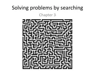
Solving Problems by Searching. Foundations for Uninformed Search Methods. Literature. S. Russell and P. Norvig. Artificial Intelligence: A Modern Approach , chapter 3. Prentice Hall, 2 nd edition, 2003.

E N D
Solving Problems by Searching Foundations for Uninformed Search Methods
Literature • S. Russell and P. Norvig. Artificial Intelligence: A Modern Approach, chapter 3. Prentice Hall, 2nd edition, 2003. • S. Amarel. On Representations of Problems of Reasoning about Actions. In: D. Michie ,editor, Machine Intelligence 3, pages 131-171, Edinburgh University Press, 1968. Reprinted in: B. Webber and N. Nilsson ,editors, Readings in Artificial Intelligence, pages 2-22, Tioga, 1981. • N. Nilsson. Principles of Artificial Intelligence, chapters 1-2. Springer, 1982. Solving Problems by Searching
Overview • Characterizing Search Problems • Searching for Solutions • Uninformed Search Strategies • Avoiding Repeated States • The Problem of Representation • Search in AND/OR-Graphs • Searching with Partial Information Solving Problems by Searching
Problems of Reasoning about Actions • aim: find a course of actions that satisfies a number of specified conditions • examples: • planning an airplane trip • planning a dinner party Solving Problems by Searching
Toy Problems concise and exact description used for illustration purposes (e.g. here) used for performance comparisons Real-World Problems no single, agreed-upon description people care about the solutions Toy Problems vs.Real-World Problems Solving Problems by Searching
Toy Problem: Missionaries and Cannibals On one bank of a river are three missionaries (black triangles) and three cannibals (red circles). There is one boat available that can hold up to two people and that they would like to use to cross the river. If the cannibals ever outnumber the missionaries on either of the river’s banks, the missionaries will get eaten. How can the boat be used to safely carry all the missionaries and cannibals across the river? Solving Problems by Searching
Search Problems • initial state • set of possible actions/applicability conditions • successor function: state set of <action, state> • successor function + initial state = state space • path (solution) • goal • goal test function or goal state • path cost function • assumption: path cost = sum of step costs • for optimality Solving Problems by Searching
initial state: all missionaries, all cannibals, and the boat are on the left bank 5 possible actions: one missionary crossing one cannibal crossing two missionaries crossing two cannibals crossing one missionary and one cannibal crossing Missionaries and Cannibals: Initial State and Actions Solving Problems by Searching
Missionaries and Cannibals: Successor Function Solving Problems by Searching
Missionaries and Cannibals: State Space 1c 1c 2c 2c 1m1c 1m1c 1m 1m 2c 2c 1c 1c 1c 1c 2m 2m 1m1c Solving Problems by Searching
goal state: all missionaries, all cannibals, and the boat are on the right bank. path cost step cost: 1 for each crossing path cost: number of crossings = length of path solution path: 4 optimal solutions cost: 11 Missionaries and Cannibals: Goal State and Path Cost Solving Problems by Searching
Oradea 71 Neamt Zerind 87 151 75 Iasi Arad 140 Sibiu 92 Fagaras 99 118 Vaslui 80 Rimnicu Vilcea 211 Timisoara 97 142 Pitesti 111 98 Lugoj 101 85 Hirsova 146 Urziceni 70 Bucharest 86 Mehadia 138 90 75 Eforie Dobreta 120 Giurgiu Craiova Real-World Problem:Touring in Romania Solving Problems by Searching
Goal Formulation • performance measure • assigns a “happiness value” to all possible world states • goal • a condition that either is or is not satisfied in a given world state; a set of world states • goal formulation • find a goal that must be true in all desirable world states, i.e. all situations in which the performance measure is high Solving Problems by Searching
Problem Formulation • problem formulation • process of deciding what actions and states to consider • granularity/abstraction level • assumptions about the environment: • static • observable • discrete • deterministic Solving Problems by Searching
Touring in Romania:Search Problem Definition • initial state: • In(Arad) • possible Actions: • DriveTo(Zerind), DriveTo(Sibiu), DriveTo(Timisoara), etc. • goal state: • In(Bucharest) • step cost: • distances between cities Solving Problems by Searching
Overview • Characterizing Search Problems • Searching for Solutions • Uninformed Search Strategies • Avoiding Repeated States • The Problem of Representation • Search in AND/OR-Graphs • Searching with Partial Information Solving Problems by Searching
Search • An agent with several immediate options of unknown value can decide what to do by first examining different possible sequences of actions that lead to states of known value, and then choosing the best sequence. • search(through the state space) for • a goal state • a sequence of actions that leads to a goal state • a sequence of actions with minimal path cost that leads to a goal state Solving Problems by Searching
Search Trees • search tree: tree structure defined by initial state and successor function • Touring Romania (partial search tree): In(Arad) In(Zerind) In(Sibiu) In(Timisoara) In(Oradea) In(Fagaras) In(Rimnicu Vilcea) In(Arad) In(Sibiu) In(Bucharest) Solving Problems by Searching
Search Nodes • search nodes: the nodes in the search tree • data structure: • state: a state in the state space • parent node: the immediate predecessor in the search tree • action: the action that, performed in the parent node’s state, leads to this node’s state • path cost: the total cost of the path leading to this node • depth: the depth of this node in the search tree Solving Problems by Searching
Expanding a Search Node function expand(node, problem) successors { } for each <action, result> inproblem.successorFn(node.state) do s new searchNode(result) s.parentNode node s.action action s.pathCost node.pathCost + problem.stepCost(action, node.state) s.depth node.depth + 1 successors successors + s returnsuccessors Solving Problems by Searching
Expanded Search Nodesin Touring Romania Example In(Arad) In(Zerind) In(Sibiu) In(Timisoara) In(Oradea) In(Fagaras) In(Rimnicu Vilcea) In(Arad) In(Sibiu) In(Bucharest) Solving Problems by Searching
Fringe Nodesin Touring Romania Example fringe nodes: nodes that have not been expanded In(Arad) In(Zerind) In(Sibiu) In(Timisoara) In(Oradea) In(Fagaras) In(Rimnicu Vilcea) In(Arad) In(Sibiu) In(Bucharest) Solving Problems by Searching
Search (Control) Strategy • search or control strategy: an effective method for scheduling the application of the successor function to generate new states • selects the next node to be expanded from the fringe • determines the order in which nodes are expanded • aim: produce a goal state as quickly as possible • examples: • LIFO-queue for fringe nodes • alphabetical ordering Solving Problems by Searching
General Tree Search Algorithm function treeSearch(problem, strategy) fringe { new searchNode(problem.initialState) } loop if empty(fringe) thenreturn failure node selectFrom(fringe, strategy) ifproblem.goalTest(node.state) then return pathTo(node) fringe fringe +expand(problem, node) Solving Problems by Searching
Key Features of the General Search Algorithm • systematic • guaranteed to not generate the same state infinitely often • guaranteed to come across every state eventually • incremental • attempts to reach a goal state step by step (rather than guessing it all at once) Solving Problems by Searching
Possible Outcomes • algorithm terminates with: • failure: no solution could be found • success: solution path was found • algorithm does not terminate Solving Problems by Searching
In(Zerind) In(Timisoara) In(Oradea) In(Rimnicu Vilcea) In(Arad) In(Sibiu) General Search Algorithm:Touring Romania Example In(Arad) In(Sibiu) In(Fagaras) In(Bucharest) fringe selected Solving Problems by Searching
Measuring Problem-Solving Performance • completeness • Is the algorithm guaranteed to find a solution when there is one? • optimality • Does the strategy find the optimal solution? • time complexity • How long does it take to find a solution? • space complexity • How much memory is need to perform the search? Solving Problems by Searching
Search Problem Complexity Measures • in theoretical Computer Science: • size of the state space graph • in Artificial Intelligence: • branching factor: maximum number of successors per node • depth of the shallowest goal node • maximum length of any path in the state space Solving Problems by Searching
Problem-Solving Performance: Examples Solving Problems by Searching
Search Cost vs. Total Cost • search cost: • time (and memory) used to find a solution • total cost: • search cost + path cost of solution • optimal trade-off point: • further computation to find a shorter path becomes counterproductive Solving Problems by Searching
Overview • Characterizing Search Problems • Searching for Solutions • Uninformed Search Strategies • Avoiding Repeated States • The Problem of Representation • Search in AND/OR-Graphs • Searching with Partial Information Solving Problems by Searching
Uninformed vs. Informed Search • uninformed search (blind search) • no additional information about states beyond problem definition • only goal states and non-goal states can be distinguished • informed search (heuristic search) • additional information about how “promising” a state is available Solving Problems by Searching
Breadth-First Search • strategy: • expand root node • expand successors of root node • expand successors of successors of root node • etc. • implementation: • use FIFO queue to store fringe nodes in general tree search algorithm Solving Problems by Searching
Breadth-First Search: Missionaries and Cannibals depth = 0 depth = 1 depth = 2 depth = 3 Solving Problems by Searching
Time and Space Complexity for Breadth-First Search • assumptions: • every search node has exactly b successors (b finite) • shallowest goal node is at finite depth d • analysis: • worst case: goal node last node at depth d • bn successors at depth n • time complexity: O(bd+1) • space complexity: O(bd+1) Solving Problems by Searching
Breadth-First Search: Evaluation Solving Problems by Searching
Exponential Complexity Solving Problems by Searching
Exponential Complexity: Important Lessons • memory requirements are a bigger problem for breadth-first search than is the execution time • time requirements are still a major factor • exponential-complexity search problems cannot be solved by uninformed methods for any but the smallest instances Solving Problems by Searching
Uniform-Cost Search • breadth-first search is optimal when all step costs are equal • uniform-cost search: • always expand the fringe node with lowest path cost first Solving Problems by Searching
Uniform-Cost Search:Touring Romania fringe Arad(0) d = 0 selected Zerind(75) Sibiu(140) Timisoara(118) d = 1 Arad(280) Oradea(291) d = 2 Arad(150) Oradea(146) Arad(236) Lugoj(229) Fagaras(239) Rimnicu Vilcea(220) Sibiu(290) Timisoara(268) Sibiu(300) Craiova(346) Zerind(217) Sibiu(297) Timisoara(340) Mehadia(299) d = 3 Zerind(225) Pitesti(317) Arad(300) Oradea(296) Arad(292) Oradea(288) d = 4 Solving Problems by Searching
Time and Space Complexity for Uniform-Cost Search • assumptions: • every search node has exactly b successors (b finite) • every step has cost ≥ ε for some positive constant ε • let C* be the cost of an optimal solution • analysis: • time complexity: O(b1+⌊C*/ε⌋) • space complexity: O(b1+⌊C*/ε⌋) Solving Problems by Searching
Uniform-Cost Search: Evaluation Solving Problems by Searching
Depth-First Search • strategy: • always expand the deepest node in the current fringe first • when a sub-tree has been completely explored, delete it from memory and “back up” • implementation: • use LIFO queue (stack) to store fringe nodes in general tree search algorithm • alternative: recursive function that calls itself on each of its children in turn Solving Problems by Searching
Depth-First Search:Missionaries and Cannibals depth = 0 depth = 1 depth = 2 depth = 3 Solving Problems by Searching
Recursive Implementation of Depth-First Search function depthFirstSearch(problem) return recursiveDFS( new searchNode(problem.initialState, problem) function recursiveDFS(node, problem) ifproblem.goalTest(node.state) thenreturn pathTo(node) foreachsuccessorin expand(node, problem) do result recursiveDFS(successor, problem) ifresult≠ failure then returnresult returnfailure Solving Problems by Searching
Time and Space Complexity for Depth-First Search • assumptions: • every search node has exactly b successors (b finite) • depth of the deepest node in the tree is m • analysis: • time complexity: O(bm) • space complexity: O(bm) Solving Problems by Searching
Depth-First Search: Evaluation Solving Problems by Searching
Depth-First Search: Finding the Optimal Path • first solution discovered may not be optimal must keep searching • continued search: • assumption: non-decreasing path costs • remember path cost of cheapest path found so far • do not expand nodes for which path cost exceeds cheapest found so far Solving Problems by Searching
Backtracking Search • a variant of depth-first search • generate only one successor at a time • each node remembers which successor to generate next • space complexity: O(m) • generate successors by modifying current state representation • must be able to undo modifications • may use even less memory (and time) Solving Problems by Searching