GEOG4650/5650 – Fall 2007 Spatial Interpolation
GEOG4650/5650 – Fall 2007 Spatial Interpolation. Triangulation Inverse-distance Kriging (optimal interpolation). What is “Interpolation”?. Predicting the value of attributes at “unsampled” sites from measurements made at point locations within the same area or region

GEOG4650/5650 – Fall 2007 Spatial Interpolation
E N D
Presentation Transcript
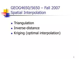
GEOG4650/5650 – Fall 2007Spatial Interpolation • Triangulation • Inverse-distance • Kriging (optimal interpolation)
What is “Interpolation”? • Predicting the value of attributes at “unsampled” sites from measurements made at point locations within the same area or region • Predicting the value outside the area - “extrapolation” • Creating continuous surfaces from point data - the main procedures
Types of Spatial Interpolation • Global or Local • Global-use every known points to estimate unknown value. • Local – use a sample of known points to estimate unknown value. • Exact or inexact interpolation • Exact – predict a value at the point location that is the same as its known value. • Inexact (approximate) – predicts a value at the point location that differs from its known value. • Deterministic or stochastic interpolation • Deterministic – provides no assessment of errors with predicted values • Stochastic interpolation – offers assessment of prediction errros with estimated variances.
Classification of Spatial Interpolation Methods Global Local Stochastic Deterministic Stochastic Deterministic Regression (inexact) Kriging (exact) Trend surface (inexact) Thiessen (exact) Density estimation(inexact) Inverse distance weighted (exact) Splines (exact)
Global Interpolation • use all available data to provide predictions for the whole area of interest, while local interpolations operate within a small zone around the point being interpolated to ensure that estimates are made only with data from locations in the immediate neighborhood. • Trend surface and regression methods
Trend Surface Analysis • Approximate points with known values with a polynomial equation. • Math equation – you don’t want to know…. • Local polynomial interpolation – uses a sample of known points, such as convert TIN to DEM
Local, deterministic methods • Define an area around the point to be predicted • finding the data points within this neighborhood • choosing a math model • evaluating the point
Thiessen Polygon (nearest neighbor) • Any point within a polygon is closer to the polygon’s known point than any other known points. • One observation per cell, if the data lie on a regular square grid, then Thiessen polygons are all equal, if irregular then irregular lattice of polygons are formed • Delauney triangulation - lines joining the data points (same as TIN - triangular irregular network)
Thiessen polygons Delauney triangulation
Example data set • soil data from Mass near the village of Stein in the south of the Netherlands • all point data refer to a support of 10x10 m, the are within which bulked samples were collected using a stratified random sampling scheme • Heavy metal concentration measured
Exercise: create Thiessen polygon for zinc concentration • Create a new project • Copy “classfiles\GEOG4650-Li\data\10-24\Soil_poll.dbf” and add it to the project. • After add the table into the project, you need to create an event theme based on this table • Go to Tools > Add XY Data and make sure the “Easting” is shown in “X” and “Northing” is in “Y”. (Don’t worry the “Unknown coordinate” • Click on OK then the point theme will appear on your project.
Exercise1) Try to plot this point data based on Zinc concentration(Try “Graduate Color” and “Graduate Symbol”)
Create a polygon theme • The next thing you need to do is provide the Thiessen polygon a boundary so that the computing of irregular polygons can be reasonable • Use ArcCatalog to create a new shapefile and name it as “Polygon.shp” • Add this layer to your current project. • Use “Editor” to create a polygon.
Notes: 1)Remember to stop Edits, otherwise your polygon theme will be under editing mode all the time2)Remember to remove the “selected” points from the “Soil_poll_data.txt”. If you are done so, your Thiessen polygons will be based on the selected points only.
Thiessen Polygon from ArcToolBox • In Arctoolbox | Analysis Tools | Proximity | Create Thiessen Polygon • Make sure the soil_poll event is the Input Features and output to your own folder. Select “All” for Output Fields.
Create Thiessen Polygons from Spatial Analyst: Set Extent and Cell Size • Go to “Spatial Analyst > Options” and click on tab and use “Polygon” as the “Analysis Mask”. • If the Analysis Mask is not set, the output layer will have rectangular shape.
Thiessen Polygon from Spatial Analyst • Select Spatial Analyst > Distance > Allocation. • In “Assign to”, select “soil_poll Event” and click OK to create cell in temporary folder.
Vector vs Raster Results • Polygons from “Analysis Tools” are vector polygons with attributes. • Polygons from “Spatial Analyst” are raster polygons with same values inside of each polygon, required to be converted to vector and NO attributes..
Zinc Concentration Plot thiessen polygons using zinc concentrations from the attribute table. Before you plot the map, trim thiessen polygons based on polygon.shp.
Inverse Distance Weighted • the value of an attribute z at some unsampled point is a distance-weighted average of data point occurring within a neighborhood, which compute: =estimated value at an unsampled point n= number of control points used to estimate a grid point k=power to which distance is raised d=distances from each control points to an unsampled point
Computing IDW 6 Z1=40 Z2=60 4 Z4=40 Z3=50 2 2 4 6 X Do you get 49.5 for the red square?
Exercise - generate a Inversion distance weighting surface and contour • Spatial Analyst > Interpolate to Raster > Inverse Distance Weighted • Make sure you have set the Output cell size to 50.
Contouring • create a contour based on the surface from IDW • Spatial Analyst | Surface Analysis | Contour
Problem - solution • Unsampled point may have a higher data value than all other controlled points but not attainable due to the nature of weighted average: an average of values cannot be lesser or greater than any input values - solution: • Fit a trend surface to a set of control points surrounding an unsampled point • Insert X and Y coordinates for the unsampled point into the trend surface equation to estimate a value at that point
Splines • draughtsmen used flexible rulers to trace the curves by eye. The flexible rulers were called “splines” - mathematical equivalents - localized • piece-wise polynomial function p(x) is
Spline - math functions • piece-wise polynomial function p(x) is • p(x)=pi(x) xi<x<xi+1 • pj(xi)=pj(xi) j=0,1,,,, • i=1,2,,,,,,k-1 i+1 x1 xk+1 x0 xk break points
Spline • r is used to denote the constraints on the spline (the functions pi(x) are polynomials of degree m or less • r = 0 - no constraints on function
Exercise: create surface from spline • have point data theme activated • Spatial Analyst | Interpolate to Raster | Spline • Define the output area and other parameters • Select “Zn” for Z Value Field and “regularized” as type and “50” for Output cell size.
Kriging • comes from Daniel Krige, who developed the method for geological mining applications • Rather than considering distances to control points independently of one another, kriging considers the spatial autocorrelation in the data
Semivariance () 20 Z1 Z2 Z3 Z4 Z5 10 20 30 35 40 50 10 20 30 40 50 Zi = values of the attribute at control points h=multiple of the distance between control points n=number of sample points
Semivariance h=1, h=2 h=3 h=4 21.88 91.67 156.25 312.50 (Z1-Z1+h)2 100 25 25 25 175 8 225 100 100 425 6 400 225 625 4 625 625 2 (Z2-Z2+h)2 (Z3-Z3+h)2 (Z4-Z4+h)2 sum 2(n-h)
semivariance • the semivariance increases as h increases : distance increases -> semivariance increases • nearby points to be more similar than distant geographical data
data no longer similar to nearby values sill range h
kriging computations • we use 3 points to estimate a grid point • again, we use weighted average =w1Z1 + w2Z2+w3Z3 = estimated value at a grid point Z1,Z2 and Z3 = data values at the control points w1,w2, and w3 = weighs associated with each control point
In kriging the weighs (wi) are chosen to minimize the difference between the estimated value at a grid point and the true (or actual) value at that grid point. • The solution is achieved by solving for the wi in the following simultaneous equations • w1(h11) + w2(h12) + w3(h13) = (h1g) w1(h12) + w2(h22) + w3(h23) = (h2g) w1(h13) + w2(h32) + w3(h33) = (h3g)
w1(h11) + w2(h12) + w3(h13) = (h1g) w1(h12) + w2(h22) + w3(h23) = (h2g) w1(h13) + w2(h32) + w3(h33) = (h3g) Where (hij)=semivariance associated with distance bet/w control points i and j. (hig) =the semivariance associated with the distance bet/w ith control point and a grid point. • Difference to IDW which only consider distance bet/w the grid point and control points, kriging take into account the variance between control points too.
Example distance 1 2 3 g Z1(1,4)=50 1 2 3 g 0 3.16 2.24 2.24 Z3(3,3)=25 0 2.24 1.00 0 1.41 Zg(2,2)=? 0 Z2(2,1)=40 w10.00+w231.6+w322.4=22.4 w131.6+w20.00+w322.4=10.0 w122.4+w222.4+w30.00=14.1 =10h h
Homework 6 – due next Friday midnight (11/2/07) • See website