An introduction to the Bootstrap method
An introduction to the Bootstrap method. Hugh Shanahan University College London November 2001. I know that it will happen, Because I believe in the certainty of chance The Divine Comedy. Outline. Origin of Statistics Central Limit Theorem Difficulties in “Standard Statistics”

An introduction to the Bootstrap method
E N D
Presentation Transcript
An introduction to the Bootstrap method Hugh Shanahan University College London November 2001 I know that it will happen, Because I believe in the certainty of chance The Divine Comedy
Outline • Origin of Statistics • Central Limit Theorem • Difficulties in “Standard Statistics” • Bootstrap - the basic idea • A simple example • Case Study I : Phylogenetic Trees • Case Study II : Bayesian Networks • Conclusions
Statistics 101 • We want the ‘average’ and ‘error’ for some variable • Time between first and second division of frog embryo • Half-life of a radioactive sample • How many days does Wimbledon get delayed by (grrr……..)
Strategy • Assuming only statistical variation • Carry out measurement “many” times • Error decreases as number of measurements increase
In fact, there’s a huge amount of statistical machinery going on with this……. Assume the Central Limit Theorem “If random samples of n observations y1, y2, …yn are drawn from a population of finite mean m and variance s2, then when n is sufficiently large, the sampling distribution of the sample mean can be approximated by a normal density with mean my = m and standard deviation sy = s/n1/2” THE MOST IMPORTANT THEOREM OF STATISTICS
Consequences of CLT • Averages taken from any distribution • (your experimental data) will have a normal • distribution • The error for such an observable will • decrease slowly as the number of • observations increase But nobody tells you how big the sample has to be..
Averages of N.D. Normal distribution c2 distribution Averages of c2 distribution
Uniform distribution Averages of U.D.
Research is more than Statistics 101 !! • Very often, we are looking at quite complicated objects, not just single variables. Even if we assume CLT, then it is not clear how to propagate the uncertainty through to the final objects we are looking at. • It is not clear when we have a large enough sample, we should do a histogram, but this may not be possible.
What the statistician sees….(or rather what they talk about) • The probability distribution rather than the data • But we just have the data ! • The bootstrap method attempts to determine • the probability distribution from the data • itself, without recourse to CLT. • The bootstrap method is not a way of reducing • the error ! It only tries to estimate it.
Basic idea of Bootstrap • Originally, from some list of data, one computes an object. • Create an artificial list by randomly drawing elements from that list. Some elements will be picked more than once. • Compute a new object. • Repeat 100-1000 times and look at the distribution of these objects.
A simple example • Data available comparing grades before and after leaving graduate school amongst 15 U.S. Universities. • Some linear correlation between grades (high incoming usually means high outgoing). r=0.776 • But how reliable is this result ?
Addendum : The Jack-knife • Jack-knife is a special kind of bootstrap. • Each bootstrap subsample has all but one of the original elements of the list. • For example, if original list has 10 elements, then there are 10 jack-knife subsamples.
How many bootstraps ? • No clear answer to this. Lots of theorems on asymptotic convergence, but no real estimates ! • Rule of thumb : try it 100 times, then 1000 times, and see if your answers have changed by much. • Anyway have NN possible subsamples
Is it reliable ? • A very very good question ! • Jury still out on how far it can be applied, but for now nobody is going to shoot you down for using it. • Good agreement for Normal (Gaussian) distributions, skewed distributions tend to more problematic, particularly for the tails, (boot strap underestimates the errors).
Case Study I : Phylogenetic Trees Get a multiple sequence alignment C1 C2 C3 S1 A A G S2 A A A S3 G G A S4 A G A Construct a Tree using your favourite method (Parsimony, ML, etc..)
How confident are we of this tree ? • For example, how confident are we that two sequences are in the same clade ? • I.E. what is the probability distribution of our confidence of the branches ? • Certainly not a problem that Stat. 101 can handle ! • Bootstrap can provide a way of determining this (first thought of by Felsenstein, 1985)
Having created an ensemble of Phylogenetic trees, one can elucidate the statistical frequency of various features of the tree. E.G. Do two sequences lie in the same clade ? Can this be used for statistical significance ? This is very much an open question !!!! (Be cautious, and assume not…...)
Case Study II : Gene expression data and Bayesian (Probabilistic) networks • A method for elucidating which genes is regulating the production of what genes. • Problem is that it is difficult to determine how reliable the edges of the network is • The bootstrap method is the favoured approach…..
Formally, we get a joint probability distribution which takes the form : P(G1,G2,….) = … x P(G3 | G1, G2 ) x … … x P(G7 | G3 ) x … etc…. More importantly, we can tell which genes directly affect which genes (e.g. G1 and G2 acting on G3) and which ones are indirect (e.g. G6 acting on G3)
But there is a problem…. • Finding the right network is an NP-hard problem. • Have to apply various heuristic techniques…. • Also, given the paucity of data it is not clear that any given connection between two genes is not a spurious correlation that will vanish with more statistics.
Summary of the Bootstrap method • Original object O (a tree, a best fit...) is computed from a “list of data” (numbers, sequences, microarray data,….). • Construct a new list, with the same number of elements, from the original list by randomly picking elements from the list. Any one element from the list can be picked any number of times. • Compute new object, call it O1 • Repeat the process many times (typically 100-1000). • The elements {O1 ,O2 , ……} are assumed to be taken from a statistical distribution, so one can compute averages, variances, etc.
Conclusions • Don’t feel bad if this went over your head ! • I’m happy to explain this again…….. • Textbook : Randomization, Bootstrap and Monte Carlo Methods in Biology, B.F.J. Manly, Chapman & Hall • Many extra subtleties, (parametric, non-parametric, random numbers) have not been discussed. • Do NOT scrimp on the explanation of this method when you are writing it up !!!