Download

1 / 54
540 likes | 724 Vues
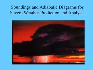
Soundings and Adiabatic Diagrams for Severe Weather Prediction and Analysis. Review. Atmospheric Soundings Plotted on Skew-T Log P Diagrams. Allow us to identify stability of a layer Allow us to identify various air masses Tell us about the moisture in a layer Help us to identify clouds

E N D
Soundings and Adiabatic Diagrams for Severe Weather Prediction and Analysis
Atmospheric Soundings Plotted on Skew-T Log P Diagrams • Allow us to identify stability of a layer • Allow us to identify various air masses • Tell us about the moisture in a layer • Help us to identify clouds • Allow us to speculate on processes occurring
Why use Adiabatic Diagrams? • They are designed so that area on the diagrams is proportional to energy. • The fundamental lines are straight and thus easy to use. • On a skew-t log p diagram the isotherms(T) are at 90o to the isentropes (q).
The information on adiabatic diagrams will allow us to determine things such as: • CAPE (convective available potential energy) • CIN (convective inhibition) • DCAPE (downdraft convective available potential energy) • Maximum updraft speed in a thunderstorm • Hail size • Height of overshooting tops • Layers at which clouds may form due to various processes, such as: • Lifting • Surface heating • Turbulent mixing
Lifting Condensation Level (LCL) • The level at which a parcel lifted dry adiabatically will become saturated. • Find the temperature and dew point temperature (at the same level, typically the surface). Follow the mixing ratio up from the dew point temp, and follow the dry adiabat from the temperature, where they intersect is the LCL.
Level of Free Convection (LFC) • The level above which a parcel will be able to freely convect without any other forcing. • Find the LCL, then follow the moist adiabat until it crosses the temperature profile. • At the LFC the parcel is neutrally buoyant.
Equilibrium Level (EL) • The level above the LFC at which a parcel will no longer be buoyant. (At this point the environment temperature and parcel temperature are the same.) • Above this level the parcel is negatively buoyant. • The parcel may still continue to rise due to accumulated kinetic energy of vertical motion. • Find the LFC and continue following the moist adiabat until it crosses the temperature profile again.
Convective Condensation Level (CCL) • Level at which the base of convective clouds will begin. • From the surface dew point temperature follow the mixing ratio until it crosses the temperature profile of sounding.
Convective Temperature (CT) • The surface temperature that must be reached for purely convective clouds to develop. (If the CT is reached at the surface then convection will be deep enough to form clouds at the CCL.) • Determine the CCL, then follow the dry adiabat down to the surface.
Mixing Condensation Level (MCL) • This represents the level at which clouds will form when a layer is sufficiently mixed mechanically. (i.e. due to turbulence) • To find the MCL determine the average potential temperature (q) and average mixing ratio (w) of the layer. Where the average q and average w intersect is the MCL.
What is Severe Weather? Tornado Hail > or = 3/4inch Wind > 50 knots
Convective Available Potential Energy (CAPE) • Remember: Area on a thermodynamic diagram is proportional to energy. • CAPE is also called buoyant energy. • CAPE on a thermodynamic diagram is the area between the parcel and the environment temperatures from the LFC to the EL • CAPE is a measure of instability
Maximum Updraft Speed • If we convert the potential energy of CAPE to a kinetic energy, we can get the maximum speed of any updraft that may develop.
Convective Inhibition (CIN) • CIN is NOT negative CAPE!!!!!! • CAPE integrates from the LFC to the EL, CIN integrates from the surface to the LFC • Is a measure of stability • Reported as an absolute value
Overcoming Convective Inhibition • A convective outbreak rarely occurs from surface heating alone! • Triggering Mechanisms for T-Storms • fronts • dry lines • sea-breeze fronts • gust fronts from other thunderstorms • atmospheric bouyancy waves • mountains
Cap Strength • Very important for severe weather to develop • Too little or no cap: happy little cumulus everywhere • Too strong of a cap: nothing happens • Just the right amount of a cap: Severe Weather
At the inversion* look at the temperature difference between the parcel and the environment.
Shear vs. CAPE • Need a balance between Shear and CAPE for supercell development • Without shear: single, ordinary, airmass thunderstorm which lasts 20 minutes • If shear is too strong: multicellular t-storms (gust front moves too fast)
Shear Just Right • 2-D equilibrium: squall line develops • 3-D equilibrium: right moving and left moving supercells A B A B L Left Mover L Right Mover
Bulk Richardson Number (BRN) BRN= CAPE 1/2Uz2 (where Uz is a measure of the vertical wind shear)
V South Hodographs • Draw wind vectors in direction they are going • This is opposite of how the wind barbs are drawn U East West Wind speed North
Storm Splitting: R and L storm cells move with mean wind but drift outward Straight Line Shear 500 700 850 900 1000
Curved Hodograph • Emphasizes one of the supercells • Veering (clockwise curve): • right moving supercells • warm air advection in northern hemisphere • Backing (counter clockwise curve): • left moving supercells • warm air advection in southern hemisphere 700 300 500 850 900 1000
Straight Line Hodograph Curved hodograph
Can be thought of as a measure of the “corkscrew” nature of the winds. Higher helicity values relate to a curved hodograph. large positive values--> emphasize right cell large negative values--> emphasize left cells Values near zero relate to a straight line hodograph. Helicity H = velocity dotted with vorticity = V • ζ = u (dyw - dzv) - v (dxw - dzu) + w (dxv - dyu)
CAPE and Helicity • Plainfield, IL tornado: • CAPE=7000 • Helicity=165 • Energy Helicity:
K Index • This index uses the values for temperature (t) and dew point temperature (td), both in oC at several standard levels. K = t850 - t 500 + td850 - t700 + td700
Vertical Totals VT = T850 - T500 • A value of 26 or greater is usually indicative of thunderstorm potential.
Cross Totals CT =T d850 - T500
Total Totals (TT) TT = VT + CT =T850 + T d850 - 2 T500
SWEAT (severe weather threat) Index SWI = 12D + 20(T - 49) + 2f8 + f5 + 125(S + 0.2) where: D=850mb dew point temperature (oC) (if D<0 then set D = 0) T = total totals (if T < 49 then set entire term = 0) f8=speed of 850mb winds (knots) f5= speed of 500mb winds (knots) S = sin (500mb-850mb wind direction) And set the term 125(S+0.2) = 0 when any of the following are not true • 850mb wind direction is between 130-250 • 500mb wind direction is between 210-310 • 500mb wind direction minus 850mb wind direction is positive • 850mb and 500mb wind speeds > 15knots
SWEAT (severe weather threat) Index SWI = 12D + 20(T - 49) + 2f8 + f5 + 125(S + 0.2)
Lifted Index (LI) • Compares the parcel with the environment at 500mb. LI = (Tenv-Tparcel)500
Best Lifted Index • Uses the highest value of qe or qwin the lower troposphere. • Use the highest mixing ratio value in combination with the warmest temperature. • SELS Lifted Index • Use the mean mixing ratio and mean q of the lowest 100mb • If using a 12z sounding add 2o • Start parcel at 50mb above the surface
Showalter Index (SI) • Compares a parcel starting at 850mb with the environment at 500mb. SI = (Tenv-Tparcel)500