Chapter 5 Randomization Methods
Chapter 5 Randomization Methods. RANDOMIZATION. Why randomize What a random series is How to randomize. Randomization (1). Rationale Reference: Byar et al (1976) NEJM 274:74-80. Best way to find out which therapy is best

Chapter 5 Randomization Methods
E N D
Presentation Transcript
RANDOMIZATION • Why randomize • What a random series is • How to randomize
Randomization (1) • Rationale • Reference: Byar et al (1976) NEJM 274:74-80. • Best way to find out which therapy is best • Reduce risk of current and future patients of being on harmful treatment
Randomization (2) Basic Benefits of Randomization • Eliminates assignment basis • Tends to produce comparable groups • Produces valid statistical tests Basic Methods Ref: Zelen JCD 27:365-375, 1974. Pocock Biometrics 35:183-197, 1979
Goal: Achieve Comparable Groups to Allow Unbiased Estimate of Treatment Beta-Blocker Heart Attack Trial Baseline Comparisons Propranolol Placebo (N-1,916) (N-1,921) Average Age (yrs) 55.2 55.5 Male (%) 83.8 85.2 White (%) 89.3 88.4 Systolic BP 112.3 111.7 Diastolic BP 72.6 72.3 Heart rate 76.2 75.7 Cholesterol 212.7 213.6 Current smoker (%) 57.3 56.8
Nature of Random Numbers and Randomness • A completely random sequence of digits is a mathematicalidealization • Each digit occurs equally frequently in the whole sequence • Adjacent (set of) digits are completely independent of one another • Moderately long sections of the whole show substantial regularity • A table of random digits • Produced by a process which will give results closely approximating • to the mathematical idealization • Tested to check that it behaves as a finite section from a • completely random series should • Randomness is a property of the table as a whole • Different numbers in the table are independent
Allocation Procedures to Achieve Balance • Simple randomization • Biased coin randomization • Permuted block randomization • Balanced permuted block randomization • Stratified randomization • Minimization method
Randomization & Balance (1) n = 100 p = ½ s = #heads V(s) = np(1-p) = 100 · ½ · ½ = 25 E(s) = n · p = 50
Randomization & Balance (2) n = 20 p = ½ E(s) = 10 V(s) = np(1-p) = 20/4 = 5
Simple Random Allocation A specified probability, usually equal, of patients assigned to each treatment arm, remains constant or may change but not a function of covariates or response a. Fixed Random Allocation • n known in advance, exactly • n/2 selected at random & assigned to Trt A, rest to Trt B b. Complete Randomization (most common) • n not exactly known • marginal and conditional probability of assignment = 1/2 • analogous to a coin flip (random digits)
Simple Randomization • Advantage: simple and easy to implement • Disadvantage: At any point in time, there may be an imbalance in the number of subjects on each treatment • With n = 20 on two treatments A and B, the chance • of a 12:8 split or worse is approximately 0.5 • With n = 100, the chance of a 60:40 split or worse is approximately 0.025 • Balance improves as the sample size n increases • Thus desirable to restrict randomization to ensure balance throughout the trial
Simple Randomization For two treatments assign A for digits 0-4 B for digits 5-9 For three treatments assign A for digits 1-3 B for digits 4-6 C for digits 7-9 and ignore 0
Simple Randomization For four treatments assign A for digits 1-2 B for digits 3-4 C for digits 5-6 D for digits 7-8 and ignore 0 and 9
Restricted Randomization • Simple randomization does not guarantee balance over time in each realization • Patient characteristics can change during recruitment (e.g. early pts sicker than later) • Restricted randomizations guarantee balance 1. Permuted-block 2. Biased coin (Efron) 3. Urn design (LJ Wei)
Permuted-Block Randomization (1) • Simple randomization does not guarantee balance in numbers during trial • If patient characteristics change with time, early imbalances • can't be corrected • Need to avoid runs in Trt assignment • Permuted Block insures balance over time • Basic Idea • Divide potential patients into B groups or blocks of size 2m • Randomize each block such that m patients are allocated to A and m to B • Total sample size of 2m B • For each block, there are possible realizations • (assuming 2 treatments, A & B) • Maximum imbalance at any time = 2m/2 = m
Permuted-Block Randomization (2) Method 1: Example • Block size 2m = 4 2 Trts A,B } = 6 possible • Write down all possible assignments • For each block, randomly choose one of the six possible arrangements • {AABB, ABAB, BAAB, BABA, BBAA, ABBA} ABAB BABA ...... Pts 1 2 3 4 5 6 7 8 9 10 11 12
Permuted-Block Randomization (3) • Method 2: In each block, generate a uniform random number for each treatment (Trt), then rank the treatments in orderTrt in Random Trt in any order Number Rank rank order A 0.07 1 A A 0.73 3 B B 0.87 4 A B 0.31 2 B
Permuted-Block Randomization (4) • Concerns - If blocking is not masked, the sequence become somewhat predictable (e.g. 2m = 4) A B A B B A B ? Must be A. A A Must be B B. - This could lead to selection bias • Simple Solution to Selection Bias • Do not reveal blocking mechanism • Use random block sizes • If treatment is double blind, no selection bias
Biased Coin Design (BCD)Efron (1971) Biometrika • Allocation probability to Treatment A changes to keep balance in each group nearly equal • BCD (p) • Assume two treatments A & B • D = nA -nB "running difference" n = nA + nB • Define p = prob of assigning Trt > 1/2 • e.g. PA = prob of assigning Trt A If D = 0, PA = 1/2 D > 0, PA = 1 - p Excess A's D < 0, PA = p Excess B's • Efron suggests p=2/3 D > 0 PA = 1/3 D < 0 PA = 2/3
Urn RandomizationWei & Lachin: Controlled Clinical Trials, 1988 • A generalization of Biased Coin Designs • BCD correction probability (e.g. 2/3) remains constant regardless of the degree of imbalance • Urn design modifies p as a function of the degree of imbalance • U(, ) & two Trts (A,B) • 0. Urn with white, red balls to start • 1. Ball is drawn at random & replaced • 2. If red, assign B If white, assign A • 3. Add balls of opposite color (e.g. If red, add white) • 4. Go to 1. • Permutational tests are available, but software not as easy.
Analysis & Inference • Most analyses do not incorporate blocking • Need to consider effects of ignoring blocks • Actually, most important question is whether we should use complete randomization and take a chance of imbalance or use permuted-block and ignore blocks • Homogeneous or Heterogeneous Time Pop. Model • Homogeneous in Time • Blocking probably not needed, but if blocking ignored, no problem • Heterogeneoous in Time • Blocking useful, intrablock correlations induced • Ignoring blocking most likely conservative • Model based inferences not affected by treatment allocation scheme. Ref: Begg & Kalish (Biometrics, 1984)
Kalish & Begg Controlled Clinical Trials, 1985 Time Trend • Impact of typical time trends (based on ECOG pts) on nominal p-values likely to be negligible • A very strong time trend can have non-negligible effect on p-value • If time trends cause a wide range of response rates, adjust for time strata as a co-variate. This variation likely to be noticed during interim analysis.
Balancing on Baseline Covariates • Stratified Randomization • Covariate Adaptive • Minimization • Pocock & Simon
Stratified Randomization (1) • May desire to have treatment groups balanced with respect to prognostic or risk factors (co-variates) • For large studies, randomization “tends” to give balance • For smaller studies a better guarantee may be needed • Divide each risk factor into discrete categories Number of strata f = # risk factors; li = number of categories in factor i • Randomize within each stratum • For stratified randomization, randomization must be restricted! Otherwise, (if CRD was used), no balance is guaranteed despite the effort.
Example Sex (M,F) and Risk (H,L) 1 2 Factors X 2 2 Levels in each 4 Strata 3 4 H L M F H L For stratified randomization, randomization must be restricted! Otherwise, (if CRD was used), no balance is guaranteed despite the effort!
Stratified Randomization (2) • Define strata • Randomization is performed within each stratum and is usually blocked • Example: Age, < 40, 41-60, >60; Sex, M, FTotal number of strata = 3 x 2 = 6 Age Male Female 40 ABBA, BAAB, … BABA, BAAB, ... 41-60 BBAA, ABAB, ... ABAB, BBAA, ...>60 AABB, ABBA, ... BAAB, ABAB, ..
Stratified Randomization (3) • The block size should be relative small to maintain balance in small strata, and to insure that the overall imbalance is not too great • With several strata, predictability should not be a problem • Increased number of stratification variables or increased number of levels within strata lead to fewer patients per stratum • In small sample size studies, sparse data in many cells defeats the purpose of stratification • Stratification factors should be used in the analysis • Otherwise, the overall test will be conservative
Comment • For multicenter trials, clinic should be a factor Gives replication of “same” experiment. • Strictly speaking, analysis should take the particular randomization process into account; usually ignored (especially blocking) & thereby losing some sensitivity. • Stratification can be used only to a limited extent, especially for small trials where it's the most useful; i.e. many empty or partly filled strata. • If stratification is used, restricted randomization within strata must be used.
Minimization Method (1) • An attempt to resolve the problem of empty strata when trying to balance on many factors with a small number of subjects • Balances Trt assignment simultaneously over many strata • Used when the number of strata is large relative to sample size as stratified randomization would yield sparse strata • A multiple risk factors need to be incorporated into a score for degree of imbalance • Need to keep a running total of allocation by strata • Also known as the dynamic allocation • Logistically more complicated • Does not balance within cross-classified stratum cells; • balances over the marginal totals of each stratum, separately
Example: Minimization Method (a) • Three stratification factors: Sex (2 levels), • age (3 levels), and disease stage (3 levels) • Suppose there are 50 patients enrolled and the 51st patient is male, age 63, and stage III • Trt A Trt B • Sex Male 16 14 • Female 10 10 • Age < 40 13 12 • 41-60 9 6 • > 60 4 6 • Disease Stage I 6 4 Stage II 13 16 • Stage III 7 4 • Total 26 24
Example: Minimization Method (b) • Method: Keep a current list of the total patients on each treatment for each stratification factor level • Consider the lines from the table above for that patient's stratification levels onlySign of • Trt A Trt B Difference • Male 16 14 + • Age > 60 4 6 - • Stage III 7 4 + • Total 27 24 2 +s and 1 -
Example: Minimization Method (c) • Two possible criteria: • Count only the direction (sign) of the difference in each category. Trt A is “ahead” in two categories out of three, so assign the patient to Trt B • Add the total overall categories (27 As vs 24 Bs). • Since Trt A is “ahead,” assign the patient to Trt B
Minimization Method (2) • These two criteria will usually agree, but not always • Choose one of the two criteria to be used for the entire study • Both criteria will lead to reasonable balance • When there is a tie, use simple randomization • Generalization is possible • Balance by margins does not guarantee overall treatment balance, or balance within stratum cells
Covariate Adaptive Allocation(Sequential Balanced Stratification)Pocock & Simon, Biometrics, 1975; Efron, Biometrika, 1971 • Goal is to balance on a number of factors but with "small" numbers of subjects • In a simple case, if at some point Trt A has more older patients than Trt B, next few older patients should more likely be given Trt B until "balance" is achieved • Several risk factors can be incorporated into a score for degree of imbalance B(t) for placing next patient on treatment t (A or B) • Place patient on treatment with probability p > 1/2 which causes the smallest B(t), or the least imbalance • More complicated to implement - usually requires a small "desk top" computer
Example: Baseline Adaptive Randomization • Assume 2 treatments (1 & 2) 2 prognostic factors (1 & 2) (Gender & Risk Group) Factor 1 - 2 levels (M & F) Factor 2 - 3 levels (High, Medium & Low Risk) Let B(t) = Wi Range (xit1, xit2) wi = weight for each factor e.g. w1 = 3 w1/w2 = 1.5 w2 = 2 xij = number of patients in ith factor and jth treatment xitj = change in xij if next patient assigned treatment t • Let P = 2/3 for smallest B(t) Pi = (2/3, 1/3) • Assume we have already randomized 50 patients • Now 51st pt. Male (1st level, factor 1) Low Risk (3rd level, factor 2)
Now determine B(1) and B(2) for patient #51.… • If assigned Treatment 1 (t = 1) • (a) Calculate B(t) (Assign Pt #51 to trt 1) t = 1 • (1) Factor 1, Level 1 • (Male) • Now Proposed • K X1K X11K • Trt Group 1 16 17 • 2 14 14 • Range =|17-14| = 3
(a) Calculate B(t) (Assign Pt #51 to trt 1) t=1 (2) Factor 2, Level 3 (Low Risk) K X2K X12K Trt Group 1 4 5 2 6 6 Range = |5-6|, = 1 * B(1) = 3(3) + 2(1) = 11
(b) Calculate B(2) (Assign Pt #51 to trt 2) t=2 (1) Factor 1, Level 1 (Male) KX1KX21K Group 1 16 16 2 14 15 Range = |16-15| = 1 (2) Factor 2, Level 3 (Low Risk) K X2k X22k Group 1 4 4 2 6 7 Range = |4-7| = 3 * B(2) = 3(1) + 2(3) = 9
(c) Rank B(1) and B(2), measures of imbalance Assign t t B(t) with probability 2 9 2/3 1 11 1/3 * Note: “minimization” would assign treatment 2 for sure
Response Adaptive Allocation Procedures • Use outcome data obtained during trial to influence allocation of patient to treatment • Data-driven • i.e. dependent on outcome of previous patients • Assumes patient response known before next patient • The goal is to allocate as few patients as possible toa seemingly inferior treatment • Issues of proper analyses quite complicated • Not widely used though much written about • Very controversial
Play-the-Winner RuleZelen (1969) • Treatment assignment depends on the outcome of previous patients • Response adaptive assignment • When response is determined quickly • 1st subject: toss a coin, H = Trt A, T = Trt B • On subsequent subjects, assign previous treatment if it was successful • Otherwise, switch treatment assignment for next patient • Advantage: Potentially more patients receive the better treatment • Disadvantage: Investigator knows the next assignment
Response Adaptive Randomization Example "Play-the-winner” Zelen (1969) JASA TRT A S S F S S S F TRT B S F Patient 1 2 3 4 5 6 7 8 9 ......
Two-armed Bandit or Randomized Play-the-Winner Rule • Treatment assignment probabilities depend on observed success probabilities at each time point • Advantage: Attempts to maximize the number of subjects on the “superior” treatment • Disadvantage: When unequal treatment numbers result, there is loss of statistical power in the treatment comparison
ECMO Example • References Michigan 1a. Bartlett R., Roloff D., et al.; Pediatrics (1985) 1b. Begg C.; Biometrika (1990) Harvard 2a. O’Rourke P., Crone R., et al.; Pediatrics (1989) 2b. Ware J.; Statistical Science (1989) 2c. Royall R.; Statistical Science (1991) • Extracoporeal Membrane Oxygenator(ECMO) • treat newborn infants with respiratory failure or hypertension • ECMO vs. conventional care
Michigan ECMO Trial • Bartlett Pediatrics (1985) • Modified “play-the-winner” • Urn model A ball ECMO B ball Standard control If success on A, add another A ball .… • Wei & Durham JASA (1978) • Randomized Consent Design • Results *sickest patient • P-Values, depending on method, values ranged .001 6 .05 6 .28
Harvard ECMO Trial (1) • O’Rourke, et al.; Pediatrics (1989) • ECMO for pulmonary hypertension • Background • Controversy of Michigan Trial • Harvard experience of standard 11/13 died • Randomized Consent Design • Two stage 1st Randomization (permuted block) switch to superior treatment after 4 deaths in worst arm 2nd Stay with best treatment
Harvard ECMO Trial (2) • Results Survival * less severe patients P = .054 (Fisher)
Multi-institutional Trials • Often in multi-institutional trials, there is a marked institution effect on outcome measures • Using permuted blocks within strata, adding institution as yet another stratification factor will probably lead to sparse cells (and potentially more cells than patients!) • Use permuted block randomization balanced within institutions • Or use the minimization method, using institution as astratification factor
Mechanics of Randomization (1) Basic Principle - “Analyze What is Randomized” * Timing • Actual randomization should be delayed until just prior to initiation of therapy • Example Alprenolol Trial, Ahlmark et al (1976) • 393 patients randomized two weeks before therapy • Only 162 patients treated, 69 alprenolol & 93 placebo
Mechanics of Randomization (2) * Operational 1. Sequenced sealed envelopes (prone to tampering!) 2. Sequenced bottles/packets 3. Phone call to central location - Live response - Voice Response System 4. One site PC system 5. Web based Best plans can easily be messed up in the implementation