Statistics A Basic Introduction and Review
Statistics A Basic Introduction and Review. Statistics Objectives. By the end of this session you will have a working understanding of the following statistical concepts: Mean, Median, Mode Normal Distribution Curve Standard Deviation, Variance Basic Statistical tests


Statistics A Basic Introduction and Review
E N D
Presentation Transcript
Statistics A Basic Introduction and Review
Statistics Objectives By the end of this session you will have a working understanding of the following statistical concepts: • Mean, Median, Mode • Normal Distribution Curve • Standard Deviation, Variance • Basic Statistical tests • Design of experiments • Hypothesis Testing and assessing significance Confidence to use in Projects/Audits
Statistics • A measurable characteristic of a sample is called a statistic • A measurable characteristic of a population, such as a mean or standard deviation, is called a parameter • Basically counting …scientifically
Sample Mean : “average” • Commonly called the average, often symbolised • Its value depends equally on all of the data which may include outliers. • It may be useful if the distribution of values is “not even” but skewed
Sample Mean : “average” Example • Our data set is: 2, 4, 8, 9, 10, 10, 10, 11 • The sample mean is calculated by taking the sum of all the data values and dividing by the total number of data values (8): • 64 divided by 8 = 4
Median : “order and middle” • The median is the halfway value through the ordered data set. Below and above this value, there will be an equal number of data values. • It gives us an idea of the “middle value” • Therefore it works well for skewed data, or data with outliers
Median : “order and middle” Example • Our Data-set is the first row of cards: ACE is 1, Jack, Queen and King are all 10 • What is the average value, what is the median value • How does the mean compare to the median value • Please repeat the exercise using the new values as below: • Our Data-set is the first row of cards: ACE is 1, Jack = 100, Queen and King are 1000
Mode: “most common” • This is the most frequently occurring value in a set of data. • There can be more than one mode if two or more values are equally common.
Mode: “most common” Example • Our Data-set is the first row of cards: ACE is 1, Jack, Queen, King are all 10 • What is the average value, what is the median value • How does the mean compare to the median value • What is the mode?
Normal Distribution: “the natural distribution” • Very easy to understand! • A continuous random variable X, taking all real values in the range is said to follow a Normal distribution with parameters µ and if it has probability density function
Normal Distribution: “the natural distribution We write • This probability density function (p.d.f.) is a symmetrical, bell-shaped curve, centred at its expected value µ. The variance is . • Many distributions arising in practice can be approximated by a Normal distribution. Other random variables may be transformed to normality. • The simplest case of the normal distribution, known as the Standard Normal Distribution, has expected value zero and variance one. This is written as N(0,1).
Normal Distribution: “the natural distribution” • Very easy to understand! No really! • Assume a gene for Height! (David not so tall!)
Normal Distribution: “the natural distribution from basic gene theory” • Assume that the gene for being Tall is Aa • So one gene from each parent is A or a • AA very tall • Aa medium height • aa shorter • Punnett Square below Frequency Distribution
Normal Distribution: “the natural distribution from basic gene theory” • Now assume that each parent has two genes for tallness • Each parent has Aa and Aa • So input from each parent would be AA or Aa or Aa or aa
Normal Distribution: “the natural distribution from basic gene theory” • Assume that there 3 genes for being Tall • AAA, Aaa, Aaa, aaa from each parent
Normal Distribution: “the natural distribution from basic gene theory” • Assume that there 3 genes for being Tall • AAA, Aaa, Aaa, aaa from each parent
Normal Distribution: “the natural distribution from basic gene theory” • AAA, Aaa, Aaa, aaa from each parent • Convert to numbers: A = 1, a =0
Worksheet: 3 Genes for Tallness • Then please plot a graph of the values versus the categories • Categories are 0,1,2,3,4,5,6
Normal Distribution: “the natural distribution from basic gene theory” • AAA, Aaa, Aaa, aaa from each parent • Convert to numbers: A = 1, a =0
Normal Distribution: “the natural distribution from basic gene theory”
Normal Distribution: “the natural distribution from basic gene theory” • Now assume that each parent has 4 genes for tallness • Each parent could give AAAA, AAAa, AAaa, Aaaa, aaaa
Frequency Distribution Chart • Notice that the frequency distribution of phenotypes like the bell shaped curve 'Normal Distribution'. • For large numbers of genes or variables each gene or factor has a small additive effect, a Normal Distribution results.
Normal Distribution: “the natural distribution from basic gene theory” Special Charactersistics 1 : • Mean. Mode and Median are the same value • Standard Deviation is 34.1% • So 68.1% of values lie within one SD of the mean • So 95.4% of values lie within 2SD of the mean
The Variance In a population, variance is the average squared deviation from the population mean, as defined by the following formula: σ2 = Σ ( Xi - μ )2 / N where σ2 is the population variance, μ is the population mean, Xi is the ith element from the population, and N is the number of elements in the population.
The Variance In a population, variance is the average squared deviation from the population mean: • Example: Take 11 cards (1 to 11), ACE = 1 to Picture card =11 • What is the average? = 6 • What is the total deviation from the mean?
The Variance In a population, variance is the average squared deviation from the population mean: • Example: Take 11 cards (1 to 11 • What is the average? = 6 • What is the total deviation from the mean? • Work out Mean minus x • Square this • Add up • Average this • The variance is ?
The Variance In a population, variance is the average squared deviation from the population mean: • Example: Take 11 cards (1 to 11 • What is the average? = 6 • What is the total deviation from the mean? • Work out Mean minus x • Square this • Add up • Average this (110 divided 11) • The variance is 10 • What is the SD?
The Standard Deviation The standard deviation is the square root of the variance. Thus, the standard deviation of a population is: σ = sqrt [ σ2 ] = sqrt [ Σ ( Xi - μ )2 / N ] where σ is the population standard deviation, σ2 is the population variance, μ is the population mean, Xi is the ith element from the population, and N is the number of elements in the population.
The Standard Deviation The standard deviation is the square root of the variance. Thus, the standard deviation of a population is: σ = sqrt [ σ2 ] = sqrt [ Σ ( Xi - μ )2 / N ] where σ is the population standard deviation, σ2 is the population variance, μ is the population mean, Xi is the ith element from the population, and N is the number of elements in the population. With our 11 cards variance was 10 So the SD is ? Square root of 10? = 3.16
The Variance and Standard Deviation 11 values Mean was 6 Variance was 10 Standard deviation = 3.16
Special Charactersistics 2: • Additionally, every normal curve (regardless of its mean or standard deviation) conforms to the following "rule". • About 68% of the area under the curve falls within 1 standard deviation of the mean. • About 95% of the area under the curve falls within 2 standard deviations of the mean. • About 99.7% of the area under the curve falls within 3 standard deviations of the mean. • Collectively, these points are known as the empirical rule or the 68-95-99.7 rule. Clearly, given a normal distribution, most outcomes will be within 3 standard deviations of the mean.
StatisticsA Basic Introduction and Review Additional Key Concepts
Simple Random Sampling A sampling method is a procedure for selecting sample elements from a population. Simple random sampling refers to a sampling method that has the following properties. • The population consists of N objects. • The sample consists of n objects. • All possible samples of n objects are equally likely to occur.
Confidence Intervals: • An important benefit of simple random sampling is that it allows researchers to use statistical methods to analyze sample results. • For example, given a simple random sample, researchers can use statistical methods to define a confidence interval around a sample mean. • Statistical analysis is not appropriate when non-random sampling methods are used. • There are many ways to obtain a simple random sample. One way would be the lottery method. Each of the N population members is assigned a unique number. The numbers are placed in a bowl and thoroughly mixed. Then, a blind-folded researcher selects n numbers. Population members having the selected numbers are included in the sample or Stat Trek!
Univariate vs. Bivariate Data • Statistical data are often classified according to the number of variables being studied. • Univariate data. When we conduct a study that looks at only one variable: eg, we say that average weight of school students. Since we are only working with one variable (weight), we would be working with univariate data. • Bivariate data. A study that examines the relationship between two variables eg height and weight
Percentiles • Assume that the elements in a data set are rank ordered from the smallest to the largest. The values that divide a rank-ordered set of elements into 100 equal parts are called percentiles. • An element having a percentile rank of Pi would have a greater value than i percent of all the elements in the set. Thus, the observation at the 50th percentile would be denoted P50, and it would be greater than 50 percent of the observations in the set. An observation at the 50th percentile would correspond to the median value in the set.
The Interquartile Range (IQR) Quartiles divide a rank-ordered data set into four equal parts. The values that divide each part are called the first, second, and third quartiles; and they are denoted by Q1, Q2, and Q3, respectively. • Q1 is the "middle" value in the first half of the rank-ordered data set. • Q2 is the median value in the set. • Q3 is the "middle" value in the second half of the rank-ordered data set.
The Interquartile Range (IQR) • The interquartile range is equal to Q3 minus Q1. • Eg: 1, 3, 4, 5, 5, 6, 7, 11. Q1 is the middle value in the first half of the data set. Since there are an even number of data points in the first half of the data set, the middle value is the average of the two middle values; that is, Q1 = (3 + 4)/2 or Q1 = 3.5. Q3 is the middle value in the second half of the data set. Again, since the second half of the data set has an even number of observations, the middle value is the average of the two middle values; that is, Q3 = (6 + 7)/2 or Q3 = 6.5. The interquartile range is Q3 minus Q1, so IQR = 6.5 - 3.5 = 3.
Shape of a distribution Here are some examples of distributions and shapes.
Correlation coefficients • Correlation coefficients measure the strength of association between two variables. The most common correlation coefficient, called the Pearson product-moment correlation coefficient, measures the strength of the linear association between variables.
How to Interpret a Correlation Coefficient • The sign and the value of a correlation coefficient describe the direction and the magnitude of the relationship between two variables. • The value of a correlation coefficient ranges between -1 and 1. • The greater the absolute value of a correlation coefficient, the stronger the linear relationship. • The strongest linear relationship is indicated by a CC of -1 or 1. • The weakest linear relationship is indicated by a CC equal to 0. • A positive correlation means that if one variable gets bigger, the other variable tends to get bigger. • A negative correlation means that if one variable gets bigger, the other variable tends to get smaller.
Scatterplots and Correlation Coefficients The scatterplots below show how different patterns of data produce different degrees of correlation.
Several points are evident from the scatterplots. • When the slope of the line in the plot is negative, the correlation is negative; and vice versa. • The strongest correlations (r = 1.0 and r = -1.0 ) occur when data points fall exactly on a straight line. • The correlation becomes weaker as the data points become more scattered. • If the data points fall in a random pattern, the correlation is equal to zero. • Correlation is affected by outliers. Compare the first scatterplot with the last scatterplot. The single outlier in the last plot greatly reduces the correlation (from 1.00 to 0.71).
What is a Confidence Interval? • Statisticians use a confidence interval to describe the amount of uncertainty associated with a sample estimate of a population parameter.
Confidence Intervals • Statisticians use a confidence interval to express the precision and uncertainty associated with a particular sampling method. A confidence interval consists of three parts. • A confidence level. • A statistic. • A margin of error. • The confidence level describes the uncertainty of a sampling method. • For example, suppose we compute an interval estimate of a population parameter. We might describe this interval estimate as a 95% confidence interval. This means that if we used the same sampling method to select different samples and compute different interval estimates, the true population parameter would fall within a range defined by the sample statistic+margin of error 95% of the time.
Confidence Level • The probability part of a confidence interval is called a confidence level. The confidence level describes the likelihood that a particular sampling method will produce a confidence interval that includes the true population parameter. • Here is how to interpret a confidence level. Suppose we collected all possible samples from a given population, and computed confidence intervals for each sample. Some confidence intervals would include the true population parameter; others would not. A 95% confidence level means that 95% of the intervals contain the true population parameter; a 90% confidence level means that 90% of the intervals contain the population parameter; and so on.
How to Interpret Confidence Intervals • Suppose that a 90% confidence interval states that the population mean is greater than 100 and less than 200. How would you interpret this statement? • Some people think this means there is a 90% chance that the population mean falls between 100 and 200. This is incorrect. Like any population parameter, the population mean is a constant, not a random variable. It does not change. The probability that a constant falls within any given range is always 0.00 or 1.00
What is an Experiment? • In an experiment, a researcher manipulates one or more variables, while holding all other variables constant. By noting how the manipulated variables affect a response variable, the researcher can test whether a causal relationship exists between the manipulated variables and the response variable.