Understanding Expected Value in Gambling and Ticketing Scenarios
This text explores the concept of expected value in different scenarios, specifically in the context of parking tickets, lottery tickets, and gambling bets. It discusses how one can make decisions based on the probabilities of getting caught without a ticket, the expected returns of playing a lottery, and the risks of a betting strategy that involves doubling bets. The underlying mathematical principles are illustrated with practical examples, showing how to calculate expected losses and gains when faced with uncertain outcomes.

Understanding Expected Value in Gambling and Ticketing Scenarios
E N D
Presentation Transcript
Expected Value Suppose it costs $2 to get a ticket from the parking ticket machine. Suppose if you are caught without a ticket, the fine is $20. Suppose that, on average, cars without tickets get caught one-quarter of the time. Then, if you don’t buy a ticket, you can expect, on the average, to pay $20 one-quarter of the times you park, or $20/4 = $5 each time you park. Of course, this is just “on the average”. But notice that it is more than the cost of buying a ticket each time.
Now suppose the probability of getting caught is p. If you do not buy a ticket, the expected result is having to pay $20 p on the average. This is more than buying the $2 ticket as long as p > 0.1. The city has to give the impression that people will be caught more than 10% of the time.
Now consider a lottery. Suppose it costs $2 to buy a ticket, 1,000,000 people play, and the prize is $1,000,000. If 1,000,000 people play, the chances of winning are 1 in 1,000,000, or p = 0.000 001. The chances of losing are q = 1-p = 1 - 0.000 001 = 0.999 999. If you win, you get $1,000,000, less $2, or $999,998. If you lose, you pay $2. The expected return is what you will get “on average”: p ($999,998) + q (-$2) = 0.000 001 ($999,998) + 0.999 999 (-$2) ≈ - $1 On the average, you will lose half the money you bet.
Of course, “on the average” means if you play a large number of times. If you buy one ticket, or ten, you can “expect” to lose all of your money. Notice that the expected return is a “weighted average”, weighted by the probabilities: p ($999,998) + q (-$2) = 0.000 001 ($999,998) + 0.999 999 (-$2) ≈ -$1
Consider the following gambling scheme: You bet $1. Somebody flips a coin. If you win, you take away $2, your original bet plus $1. If you lose, you lose your $1 and bet $2 on the next toss. • If you win, you get $4, but you’ve already bet • $1 + $2 = $3, so you walk away with $1. If you lose, you lose your $2 and you bet $4 on the next toss. • If you win, you get $8, but you’ve already bet • $1+$2+$4=$7, • so you walk away with $1.
Continuing like this, doubling the bet each time you lose, you always eventually win $1. What’s the catch? You have to have a lot of money. Suppose you have $1023. That means you can double the bet nine times. • You win $1 each round. • UNLESS • you lose the toss ten times in a row.
Losing ten times in a row will occur only rarely. The probability is q = (1/2)10. But, when you lose, you lose BIG. If you lose the tenth toss, you lose $1+$2+ … + $512 = $1023. What is the expectation? It is the weighted average: • p ($1) + q (-$1023) • = (1- (1/2)10)($1) + (1/2)10(-$1023) • = 0.
Jim flips a coin until it comes up heads three times in a row. Then, pointing out that four heads in a row is pretty rare, he offers to bet that it will be heads the next time, except that he wants Sam, who is making the “safer” bet that it will be tails, to give him odds of 2 to 1. In other words, if the next toss is tails, Jim pays $1, but if it is heads, Sam must pay him $2. What is his expectation? The basic point is that the next toss will still be heads half the time and tails half the time. So p = q = ½. Jim’s expectation is p ($2) + q (-$1) = ½ ($2) – ½ ($1) = $0.50
Voltaire 1694 – 1778
Each individual has genetic information encoded in DNA molecules, one strand inherited from each parent. Each DNA molecule is a double helix, but for our purposes, it can be regarded as a long chain. Along the chain, information is coded using four chemical “letters”, A, C, G, and T. Much of the chain seems to be irrelevant, but certain sections, or “loci” are the locations of genes. Genes contain the information necessary for specific purposes in the construction or operation of the body. Many genes come in different versions, or “alleles”. For a given gene, each individual has two alleles, one on each of the two DNA strands. They might be the same or they might be different. The individual’s genetic makeup is determined by which alleles are present at each locus.
The Eastern gray squirrel has a locus which controls its colour. There are two alleles of the corresponding gene, call them M and m. A squirrel with two m alleles is said to have genotype mm, and it is gray. A squirrel with genotype mM or MM is black.
The m allele is said to be “recessive”, which means that it has an effect only when both alleles are m. The M allele is “dominant”, meaning that it is “expressed” if even one of the alleles is an M. Consider a population in which one third of the alleles are m and two thirds are M. We say that the “frequencies” of m and M in the population are p = 1/3 and q = 2/3, respectively. When a new squirrel is born, we think of its two alleles as being chosen randomly from the population. The probability of getting an m allele is p = 1/3 and the probability of getting an M allele is q = 2/3. The probability of getting two m alleles is p2 = 1/9 and the probability of getting two M alleles is q2 = 4/9. The probability of getting one m allele and one M allele is given by the binomial theorem: ( ) 2 1 pq = 2 (1/3)(2/3) = 4/9.
The allele frequencies in this population are p = 1/3 and q = 2/3 for the m and M alleles, respectively. The genotype frequencies are as follows: Genotype mm Mm MM 1/9 4/9 4/9 p2 2pq q2 Allele Frequencies m M 1/3 2/3 p q The recessive m allele has frequency 1/3 in the population, and yet the corresponding gray squirrel makes up only 1/9 of the population.
Another example is the ABO blood type polymorphism. Here there are three alleles: A, B, and O. The O allele is recessive. That means that only OO individuals have type O blood. The A and B alleles are “codominant”. This means that an individual with genotype AO or AA has type A blood, while an individual with genotype BO or BB has type B blood. An individual with genotype AB is neither A nor B, but has type AB blood.
Another example is tongue rolling in humans. It is controlled by a single locus with two alleles, r and R. The r allele is recessive. Only rr individuals are unable to roll their tongues. Suppose we know the allele frequencies in the population. That is, suppose the frequency of R is p and the frequency of r is q. As before, we see that the frequency of the rr genotype is q2. It is possible to use this information in reverse: we can observe the frequency of the rr genotype. That allows us to estimate q2. From this we can find q and hence p and then the other genotype frequencies.
Hardy-Weinberg Equilibrium — named after a mathematician named Hardy and a geneticist named Weinberg. It assumes that mating is random, i.e., in mathematical terms, that the probability of getting allele A equals the frequency p of A in the population. In genetics books, it is often stated in terms of a population in which there is NO selection, NO immigration, NO mutation, etc.
Then, as we have already seen, if there are two alleles, A and B, with frequencies p and q, respectively, the genotype frequencies in the offspring are: Genotype AA AB BB p2 2pq q2 What are the allele frequencies in the offspring? The individuals having genotype AA have a frequency in the population of p2. The individuals having genotype AB have a frequency in the population of 2pq. The AA individuals have only A alleles, while the AB individuals have half A and half B. The overall proportion of A alleles in the offspring is p2 + ½ 2pq = 1 = p(p + q) = p = p2 + pq
The Hardy-Weinberg Principle Assuming that mating is random, the allele frequencies among the offspring will be the same as those among the parents. Moreover, the genotype frequencies will be given by the formulas discussed earlier: Genotype AA AB BB p2 2pq q2
This too can be used in reverse. If a population is not in Hardy-Weinberg equilibrium, i.e., if its genotype frequencies do not follow the expected pattern, then we can infer that mating is NOT random. Then we can look to see what is causing the discrepancy.
Example: Suppose a population has two alleles A and B at a locus, and the genotype frequencies are observed to be as follows: AA AB BB 1/9 23/36 1/4 We expect that the frequency of AA should equal p2, so p should be the square-root of 1/9, or 1/3. Similarly, the frequency of BB should equal q2, so q should be the square-root of 1/4, or 1/2. But we expect p + q = 1, and 1/3 + ½ = 5/6 ≠ 1. The discrepancy suggests that there might be selection or immigration, etc., in this population.
Selection Suppose there are two alleles A and B at a locus, with frequencies p and q, respectively. Then we expect the genotypes to have the usual frequencies: AA AB BB p2 2pq q2 But suppose there is something disadvantageous about the BB genotype. As an extreme example, consider the case in which BB individuals do not survive. In this case, B is called a “recessive lethal” allele. In the surviving population, all the B alleles that went to BB individuals will be lost. This reduces the frequency of B in the population.
This is an example of natural selection. The disadvantage experienced by the BB individuals results in a reduction of the proportion of the B allele. A population experiencing selection violates the Hardy-Weinberg assumption because, in effect, the BB individuals produced randomly are not given an equal opportunity to survive. In real life, the difference is usual less drastic, but different genotypes can behave differently in ways that affect their survival. A famous example is the peppered moth.