Regression Analysis

1. Regression Analysis Intro to OLS Linear Regression

2. Regression Analysis • Defined as the analysis of the statistical relationship among variables • In it’s simplest form there are only two variables: • Dependent or response variable (labeled as Y) • Independent or predictor variable (labeled as X)

3. Statistical Relationships- A warning • Be aware that as with correlation and other measures of statistical association, a relationship does not guarantee or even imply a causality between the variables • Also be aware of the difference between a mathematical or functional relationship based upon theory and a statistical relationship based upon data and its imperfect fit to a mathematical model

4. Simple Linear Regression • The basic function for linear regression is Y=f(X) but the equation typically takes the following form: • Y=α+βX+ε • α - Alpha – an intercept component to the model that represents the models value for Y when X=0 • β - Beta – a coefficient that loosely denotes the nature of the relationship between Y and X and more specifically denotes the slope of the linear equation that specifies the model • ε - Epsilon – a term that represents the errors associated with the model

5. Example • i in this case is a “counter” representing the ith observation in the data set

6. Accompanying Scatterplot

7. Accompanying Scatterplot with Regression Equation

8. What does the additional info mean? • α - Alpha – 138 cones • β - Beta – -16 cones/$1 increase in cost • ε - Epsilon – still present and evidenced by the fact that the model does not fit the data perfectly • R2 - a new term, the Coefficient of Determination - a value of 0.71 is pretty good considering that the value is scaled between 0 and 1 with 1 being a model with a perfect agreement with the data

9. Coefficient of Determination • In this simple example R2 is indeed the square of R • Recall that R is often the symbol for the Pearson Product Moment Correlation (PPMC) which is a parametric measure of association between two variables • R (X,Y) = -0.84 in this case –0.84^2=0.71

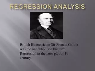
10. A Digression into History • Adrien Legendre- the original author of “the method of least squares”, published in 1805

11. The guy that got the credit- • Carl-Fredrick- the “giant” of early statistics • AKA – Gauss – published the theory of least squares in 1821

12. Back on Topic – a recap of PPMC or r • From last semester: • The PPMC coefficient is essentially the sum of the products of the z-scores for each variable divided by the degrees of freedom • Its computation can take on a number of forms depending on your resources

13. What it looks like in equation form: Mathematically Simplified Computationally Easier • The sample covariance is the upper center equation without the sample standard deviations in the denominator • Covariance measures how two variables covary and it is this measure that serves as the numerator in Pearson’s r

14. Take home message • Correlation is a measure of association between two variables • Covariance is a measure of how the two variables vary with respect to one another • Both of these are parametrically based statistical measures – note that PPMC is based upon z-scores • Z-scores are based upon the normal or Gaussian distribution - thus these measures as well as linear regression based upon the method of least squares is predicated upon the assumption of normality and other parametric assumptions

15. OLS defined • OLS stands for Ordinary Least Squares • This is a method of estimation that is used in linear regression • Its defining and nominal criteria is that it minimizes the errors associated with predicting values for Y • It uses a least squares criterion because a simple “least” criterion would allow positive and negative deviations from the model to cancel each other out (using the same logic that is used for computations of variance and a host of other statistical measures)

16. The math behind OLS • Recall that the linear regression equation for a single independent variable takes this form: Y=α+βX+ε Since Y and X are known for all I and the error term is immutable, minimizing the model errors is really based upon our choice of alpha and beta

17. is this under the condition that S is the total sum of squared deviations from i =1 to n for all Y and X for an alpha and beta This The correct alpha and beta to minimize S can be found by taking the partial derivative for alpha and beta by setting each of them equal to zero for the other, yielding for alpha, and for beta which can be further simplified to for alpha and for beta

18. Refer to page 436 for the the text’s more detailed description of the computations for solving for alpha and beta Given these, we can easily solve for the more simple alpha via algebra and since X(bar) is the sum of all X(I) from 1 to n diveded by n and the same can be said for Y(bar) we are left with is Since the mean of both X and Y can be obtained from the data, we can calculate the intercept or alpha very simply if we know the slope or beta

19. Once we have a simple equation for alpha, we can plug it into the equation for beta and then solve for the slope of the regression equation Multiply by n and you get isolate beta and we have

20. Alpha or the regression intercept Beta or the regression slope

21. Given this info, let’s • Head over to the lab and get some hand’s on practice using the small and relatively simple ice cream sale’s data set • We will cover the math behind the coefficient of determination on Thursday and introduce regression with multiple independent variables