Introduction to Quasirandomness: Exploring Pseudorandomness and Quasirandom Analogues in Computational Science
Dive into the world of quasirandomness and pseudorandomness in computational science. Discover how quasirandom elements imitate random objects' properties, leading to the development of (quasi)-Monte Carlo methods. Learn why studying quasirandomness can enhance numerical integration and more.

Introduction to Quasirandomness: Exploring Pseudorandomness and Quasirandom Analogues in Computational Science
E N D
Presentation Transcript
Quasirandomness Benjamin Doerr Max-Planck-Institut für Informatik Saarbrücken
= ¯ ¯ ¯ ¯ 1 2 + j j j j ( ( ) ) j j j j ( ( j j ( j j ) ) ) l l l P P R R R R P P O O P P " ¡ ¡ \ \ v v o o o g = = ¯ ¯ ¯ ¯ Introduction to Quasirandomness • Pseudorandomness: • Aim: Have something look completely random • Example: Pseudorandom numbers shall look random independent of the particular application. • Quasirandomness: • Aim: Imitate a particular property of a random object. • Example: Low-discrepancy point sets • A random point set P is evenly distributed in [0,1]2: For all axis-parallel rectangles R, • Quasirandom analogue: There are point sets P such that holds for all R • Leads to (Quasi)-Monte-Carlo methods Benjamin Doerr
Why Study Quasirandomness? • Basic research: Is it truely the randomness that makes a random object useful, or something else? • Example numerical integration: Random sample points are good because of their sublinear discrepancy (and ‘not’ because they are random) • Learn from the random object and make it better (custom it to your application) without randomness! • Combine random and quasirandom elements: What is the right dose of randomness? Benjamin Doerr
Outline of the Talk • Part 0: Introduction to Quasirandomness [done] • Quasirandom: Imitate a particular aspect of randomness • Part 1: Quasirandom random walks • also called “Propp machine” or “rotor router model” • Part 2: Quasirandom rumor spreading • the right dose of randomness? Benjamin Doerr
Part 1: Quasirandom Random Walks • Reminder: Random Walk • How to make it quasirandom? • Three results: • Cover times • Discrepancies: Massive parallel walks • Internal diffusion limited aggregation (physics) Benjamin Doerr
Reminder: Random Walks • Rule: Move to a neighbor chosen at random Benjamin Doerr
Quasirandom Random Walks • Simple observation: If the random walk visits a vertex many times, then it leaves it to each neighbor approximately equally often • n visits to a vertex of constant degree d: n/d + O(n1/2) moves to each neighbor. • Quasirandomness: Ensure that neighbors are served evenly! Benjamin Doerr
Quasirandom Random Walks • Rule: Follow the rotor. Rotor updates after each move. Benjamin Doerr
Quasirandom Random Walks • Simple observation: If the random walk visits a vertex many times, then it leaves it to each neighbor approx. equally often • n visits to a vertex of constant degree d: n/d + O(n1/2) moves to each neighbor. • Quasirandomness: Ensure that neighbors are served evenly! • Put a rotor on each vertex, pointing to its neighbors • The quasirandom walk moves in the rotor direction • After each step, the rotor turns and points to the next neighbor (following a given permutation of the neighbors) Benjamin Doerr
Quasirandom Random Walks • Other names • Propp machine (after Jim Propp) • Rotor router model • Deterministic random walk • Some freedom in the design • Initial rotor directions • Order, in which the rotors serve the neighbors • Also: Alternative ways to ensure fairness in serving the neighbors Fortunately: No real difference Benjamin Doerr
Result 1: Cover Times • Cover time: How many step does the (quasi)random walk need to visit all vertices? • Classical result [AKLLR’79]: For all graphs G=(V,E) and all vertices v, the expected time a random walk started in v needs to visit all vertices, is at most 2 |E|(|V|-1). • Quasirandom [D]: For all graphs, starting vertices, initial rotor directions and rotor permutations, the quasirandom walk needs at most 2|E|(|V|-1) steps to visit all vertices. • Note: Same bound, but ‘sure’ instead of ‘expected’. Benjamin Doerr
Result 2: Discrepancies • Model: Many chips do a synchronized (quasi)random walk • Discrepancy: Difference between the number of chips on a vertex at a time in the quasirandom model and the expected number in the random model Benjamin Doerr
Example: Discrepancies on the Line Random Walk (Expectation): 19 2.375 4.75 7.125 9.5 9.5 7.125 9.5 4.75 2.375 Quasirandom: 19 2 5 8 9 9 10 6 5 3 But: You’ll never have more than 2.29 [Cooper, D, Spencer, Tardos] A discrepancy > 1! Difference: -0.375 0.25 0.875 -0.5 -0.5 -1.125 0.5 0.25 0.625 Benjamin Doerr
Result 2: Discrepancies • Model: Many chips do a synchronized (quasi)random walk • Discrepancy: Difference between the number of chips on a vertex at a time in the quasirandom model and the expected number in the random model • Cooper, Spencer [CPC’06]: If the graph is an infinite d-dim. grid, then (under some mild conditions) the discrepancies on all vertices at all times can be bounded by a constant (independent of everything!) • Note: Again, we compare ‘sure’ with expected • Cooper, D, Friedrich, Spencer [SODA’08]: Fails for infinite trees • Open problem: Results for any other graphs Benjamin Doerr
Result 3: Internal Diffusion Limited Aggregation • Model: • Start with an empty 2D grid. • Each round, insert a particle at ‘the center’ and let it do a (quasi)random walk until it finds an empty grid cell, which it then occupies. • What is the shape of the occupied cells after n rounds? • 100, 1600 and 25600 particles in the random walk model: [Moore, Machta] Benjamin Doerr
Result 3: Internal Diffusion Limited Aggregation • Model: • Start with an empty 2D grid. • Each round, insert a particle at ‘the center’ and let it do a (quasi)random walk until it finds an empty grid cell, which it then occupies. • What is the shape of the occupied cells after n rounds? • With random walks: • Proof: outradius – inradius = O(n1/6) [Lawler’95] • Experiment: outradius – inradius ≈ log2(n) [Moore, Machta’00] • With quasirandom walks: • Proof: outradius – inradius = O(n1/4+eps) [Levine, Peres] • Experiment: outradius – inradius < 2 Benjamin Doerr
Summary Quasirandom Walks • Model: • Follow the rotor and rotate it • Simulates: Random walks leave each vertex in each direction roughly equally often • Results: Surprising good simulation (or “better”) • Graph exploration in 2|E|(|V|-1) steps • Many chips: For grids (but not trees), we have the same number of chips on each vertex at all times as expected in the random walk (apart from constant discrepancy) • IDLA: Almost perfect circle. Benjamin Doerr
Part 2: Quasirandom Rumor Spreading • Reminder: Randomized Rumor Spreading • same as in the talk by Thomas Sauerwald • Quasirandom Rumor Spreading • Purely deterministic: Poor • With a little bit of randomness: Great![simpler and better than randomized] • “The right dose of randomness”? Benjamin Doerr
Randomized Rumor Spreading • Model (on a graph G): • Start: One node is informed • Each round, each informed node informs a neighbor chosen uniformly at random • Broadcast time T(G): Number of rounds necessary to inform all nodes (maximum taken over all starting nodes) Round 4: Each informed node informs a random node Round 5: Let‘s hope the remaining two get informed... Round 2: Each informed node informs a random node Round 3: Each informed node informs a random node Round 1: Starting node informs random node Round 0: Starting node is informed Benjamin Doerr
Randomized Rumor Spreading • Model (on a graph G): • Start: One node is informed • Each round, each informed node informs a neighbor chosen uniformly at random • Broadcast time T(G): Number of rounds necessary to inform all nodes (maximum taken over all starting nodes) • Application: • Broadcasting updates in distributed databases • simple • robust • self-organized Benjamin Doerr
Randomized Rumor Spreading • Model (on a graph G): • Start: One node is informed • Each round, each informed node informs a neighbor chosen uniformly at random • Broadcast time T(G): Number of rounds necessary to inform all nodes (maximum taken over all starting nodes) • Results [n: Number of nodes]: • Easy: For all graphs G, T(G) ≥ log(n) • Frieze, Grimmet: T(Kn) = O(log(n)) w.h.p. • Feige, Peleg, Raghavan, Upfal: T({0,1}d) = O(log(n)) w.h.p. • Feige et al.: T(Gn,p) = O(log(n)) w.h.p., p > (1+eps)log(n)/n Benjamin Doerr
Deterministic Rumor Spreading? • As above except: • Each node has a list of its neighbors. • Informed nodes inform their neighbors in the order of this list. • Problem: Might take long... • Here: n-1 rounds . 1 2 3 4 5 6 List: 2 3 4 5 6 3 4 5 6 1 4 5 6 1 2 5 6 1 2 3 6 1 2 3 4 1 2 3 4 5 Benjamin Doerr
Semi-Deterministic Rumor Spreading • As above except: • Each node has a list of its neighbors. • Informed nodes inform their neighbors in the order of this list, but start at a random position in the list Benjamin Doerr
Semi-Deterministic Rumor Spreading • As above except: • Each node has a list of its neighbors. • Informed nodes inform their neighbors in the order of this list, but start at a random position in the list • Results (1): Benjamin Doerr
Semi-Deterministic Rumor Spreading • As above except: • Each node has a list of its neighbors. • Informed nodes inform their neighbors in the order of this list, but start at a random position in the list • Results (1): The log(n) bounds for • complete graphs, • random graphs Gn,p, p > (1+eps) log(n), • hypercubes still hold... Benjamin Doerr
Semi-Deterministic Rumor Spreading • As above except: • Each node has a list of its neighbors. • Informed nodes inform their neighbors in the order of this list, but start at a random position in the list • Results (1): The log(n) bounds for • complete graphs, • random graphs Gn,p, p > (1+eps) log(n), • hypercubes still hold independent from the structure of the lists [D, Friedrich, Sauerwald (SODA’08)] Benjamin Doerr
Semi-Deterministic Rumor Spreading • Results (2): • Random graphs Gn,p, p = (log(n)+log(log(n)))/n: • fully randomized: T(Gn,p) = Θ(log(n)2) w.h.p. • semi-deterministic: T(Gn,p) = Θ(log(n)) w.h.p. • Complete k-regular trees: • fully randomized: T(G) = Θ(k log(n)) w.h.p. • semi-deterministic: T(G) = Θ(k log(n)/log(k)) w.p.1 • Algorithm Engineering Perspective: • need fewer random bits • easy to implement: Any implicitly existing permutation of the neighbors can be used for the lists Benjamin Doerr
The Right Dose of Randomness? • Results indicate that the right dose of randomness can be important! • Alternative to the classical “everything independent at random” • May-be an interesting direction for future research? • Related: • Dependent randomization, e.g., dependent randomized rounding: • Gandhi, Khuller, Partharasathy, Srinivasan (FOCS’01+02) • D. (STACS’06+07) • Randomized search heuristics: Combine random and other techniques, e.g., greedy • Example: Evolutionary algorithms • Mutation: Randomized • Selection: Greedy (survival of the fittest) Benjamin Doerr
Summary • Quasirandomness: • Simulate a particular aspect of a random object • Surprising results: • Quasirandom walks • Quasirandom rumor spreading • For future research: • Good news: Quasirandomness can be analyzed (in spite of ‘nasty’ dependencies) • Many open problems • “What is the right dose of randomness?” Thanks! Benjamin Doerr