Download
1 / 15
150 likes | 474 Vues
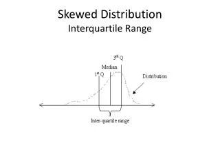
Describing a Skewed Distribution Numerically. Median IQR Inter-Quartile Range Outliers Boxplots. Barry Bonds (Again). A histogram of the data shows the distribution to be right skewed with one possible unusual season (73). Finding a “typical” value.

E N D
Describing a Skewed Distribution Numerically Median IQR Inter-Quartile Range Outliers Boxplots
Barry Bonds (Again) A histogram of the data shows the distribution to be right skewed with one possible unusual season (73)
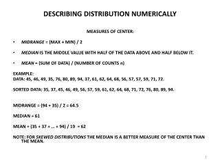
Finding a “typical” value • When a distribution is skewed or has unusually high or low values, we need to choose a measure of center that is resistant to these features. • The Median, ,is the middle value in a set of ordered data. • To find the median we must first put the data in order. 16 19 24 25 25 33 33 34 34 37 37 40 42 46 49 73
16 19 24 25 25 33 33 34 34 37 37 40 42 46 49 73 • Two possible situations may exist… • We may have an odd number of data pieces 16 19 24 25 25 33 33 34 34 37 37 40 42 46 49 (this is Barry Bonds data without the 73 season) • To find the middle position, find: n+1 for our data 15 + 1 = 8 2 2 So the “middle” number is in the 8th position 16 19 24 25 25 33 33 34 34 37 37 40 42 46 49 34
16 19 24 25 25 33 33 34 34 37 37 40 42 46 49 73 • The other possibility is for the number of pieces of data to be even. • Now we have two middle values!!! To find the position of the first one: n 2 • For our data set this means the first middle value is 16/2 = 8th. The second middle value is the next piece of data: position 9th for out data.
Once we find these two pieces of data, we need to find the average of these values 16 19 24 25 25 33 33 34 34 37 37 40 42 46 49 73 • Now we find the average of these two values (34 +34)/2 = 34. So the median is 34 • We use the median as our measure of center when our distribution is skewed or we have unusual values. • This is because the median is concerned only about placement in an ordered set of data, not the values of the data.
IQR as measure of spread • To find our measure of spread we need to divide our data set into quartiles (4 equal pieces) • Once we have found the median (this divided the data into two equal parts), we can divide these two parts again in half by finding the median of the lower half and the median of the upper half.
16 19 24 25 25 33 33 34 34 37 37 40 42 46 49 7325 34 41 Q1 Median (Q2) Q3 • To find Q1, we’ll simply find the median of the lower half 16 19 24 25 25 33 33 34 • The number of data pieces, “n” is even so find the two middle values and then find their average. • (25 + 25)/2 = 25, thus Q1 is 25. • Find Q3 in the same way, but use the upper half of the data. 34 37 37 40 42 46 49 73 • Again, n=8, so (40 + 42)/2 = 41, Q3 is 41 • The measure of spread, IQR measures the “middle 50% of the data”, the area between Q1 and Q3 • Thus, the IQR= Q3 – Q1 = 41 – 25 = 16
16 19 24 25 25 33 33 34 34 37 37 40 42 46 49 7325 34 41 Q1 Median (Q2) Q3 • 5-number summary: • The 5-number summary consists of: • Min, Q1, Median, Q3, Max • We only have to add the Minimum value and the Maximum value to the values we have already found. • So the 5-number summary is: • Min Q1 Median Q3 Max 16 25 34 41 73
Outliers • We can check the data set for unusual values by finding both an lower and upper bound. Any values beyond these boundaries are considered outliers. • To find the boundaries: • LB = Q1 - 1.5(IQR) UB = Q3 + 1.5(IQR) 25 – 1.5(16) 41 + 1.5(16) 1 65 • There is one season in which Barry Bonds hit more than 65 home runs. Since this season’s number of home runs (73) is greater than the upper bound, we would consider it to be an outlier. • There are no outliers on the lower side of the distribution.
Creating a Box Plot/Modified Box Plot • To create one last graphical picture for our data, we will create a box plot/modified box plot. • All we need to create this picture is the 5-number summary.
Box Plot • To create a box plot, use either a horizontal or vertical scale for the variable. • At each value of the 5-number summary put a point. • Enclose the “middle” 50%---Q1 to Q3 with a box, and draw a line in the box to indicate where the median lies. • Finally, extend a line to both the minimum and maximum value. (these are the “whiskers)
Modified Box Plot • To create the modified box plot, follow the directions for the box plot with the following exception. • Mark any outliers with an asterisk. The whiskers will not extend to these values. • Find the first value inside the boundary and extend the whisker to this point instead.
Resources • Practice of Statistics: pg 35-42 • Homework: 1.2 (you can now complete all of this homework)