Download
1 / 49
490 likes | 792 Vues
Randomized algorithms for the least-squares approximation problem. Petros Drineas Rensselaer Polytechnic Institute Computer Science Department. For papers, etc. drineas. Overview. L 2 regression algorithms Overview of well-known numerical analysis algorithms,

E N D
Randomized algorithms for the least-squares approximation problem Petros Drineas Rensselaer Polytechnic Institute Computer Science Department For papers, etc. drineas
Overview • L2 regression algorithms • Overview of well-known numerical analysis algorithms, • Measuring the “importance” of each constraint • A fast randomized algorithm • The column subset selection problem (CSSP) • Deterministic and Randomized Algorithms • Summary and an open problem
Model y(t) (unknown) as a linear combination of d basis functions: A is an n x d “design matrix” (n >> d): In matrix-vector notation, Problem definition and motivation In many applications (e.g., statistical data analysis and scientific computation), one has n observations of the form:
Least-norm approximation problems Recall a linear measurement model: In order to estimate x, solve:
Application: data analysis in science • First application: Astronomy Predicting the orbit of the asteroid Ceres (in 1801!). Gauss (1809) -- see also Legendre (1805) and Adrain (1808). First application of “least squares optimization” and runs in O(nd2) time! • Data analysis: Fit parameters of a biological, chemical, economical, physical (astronomical), social, internet, etc. model to experimental data.
Norms of common interest Let y = b and define the residual: Least-squares approximation: Chebyshev or mini-max approximation: Sum of absolute residuals approximation:
Lp regression problems We are interested in over-constrained Lp regression problems, n >> d. Typically, there is no xsuch that Ax = b. Want to find the “best” x such that Ax ≈ b. We want to sample a subset of constraints and work only on these constraints.
Projection of b on the subspace spanned by the columns of A Pseudoinverse of A Exact solution to L2 regression Cholesky Decomposition: If A is full rank and well-conditioned, decompose ATA = RTR, where R is upper triangular, and solve the normal equations: RTRx = ATb. QR Decomposition: Slower but numerically stable, esp. if A is rank-deficient. Write A = QR, and solve Rx = QTb. Singular Value Decomposition: Most expensive, but best if A is very ill-conditioned. Write A = UVT, in which case: xOPT = A+b = V-1UTb. Complexity is O(nd2) , but constant factors differ.
Questions … Let p=2. Approximation algorithms: Can we approximately solve L2 regression faster than “exact” methods? Core-sets (or induced sub-problems): Can we find a small set of constraints such that solving the L2 regression on those constraints gives an approximation to the original problem?
Randomized algorithms for Lp regression Note: Clarkson ’05 gets a (1+)-approximation for L1 regression in O*(d3.5/4) time. He preprocessed [A,b] to make it “well-rounded” or “well-conditioned” and then sampled.
Algorithm 1: Sampling for L2 regression • Algorithm • Fix a set of probabilities pi, i=1…n, summing up to 1. • Pick the i-th row of A and the i-th element of b with probability • min {1, rpi}, • and rescale both by (1/min{1,rpi})1/2. • Solve the induced problem. Note:in expectation, at most r rows of A and r elements of b are kept.
scaling to account for undersampling Sampling algorithm for L2 regression sampled “rows” of b sampled rows of A
Our results for p=2 If the pi satisfy a condition, then with probability at least 1-, (A): condition number of A The sampling complexity is
0 0 Let 1¸2¸ … ¸ be the entries of . Exact computation of the SVD takes O(min{mn2 , m2n}) time. The top k left/right singular vectors/values can be computed faster using Lanczos/Arnoldi methods. SVD: formal definition : rank of A U (V): orthogonal matrix containing the left (right) singular vectors of A. S: diagonal matrix containing the singular values of A.
Notation U(i): i-th row of U : rank of A U: orthogonal matrix containing the left singular vectors of A.
lengths of rows of matrix of left singular vectors of A Condition on the probabilities Thecondition that the pi must satisfy is, for some (0,1] : • Notes: • O(nd2) time suffices (to compute probabilities and to construct a core-set). • As decreases, the number of rows that we need to keep increases proportionally to 1/. • Important question: • Is O(nd2) necessary?Can we compute the pi’s, or construct a core-set, faster?
Condition on the probabilities, cont’d • Important: Sampling process must NOT loose any rank of A. • (Since pseudoinverse will amplify that error!) • Notation: • S is an r £ n matrix that samples and rescales a small number of rows of A and elements of b. • Each row of S has exactly one non-zero element (corresponding to the selected row of A); this non-zero element is set to the “rescaling value.”
Critical observation sample & rescale sample & rescale
Critical observation, cont’d SUA is approx. orthogonal • The approx. orthogonality of SUA allows us to prove that: • The left singular vectors of SA are (approx.) SUA. • The singular values of SA are (approx.) equal to the singular values of A. • A corollary of the above is that SA is full rank.
What if we are allowed to keep non-uniform samples of the rows of an orthogonal matrix (scaled appropriately)? Then, in our case (n >> d), we can prove that: (Similar arguments in Frieze, Kannan, and Vempala ’98 & ‘04, D. and Kannan ’01, D. Kannan, and Mahoney ’06, Rudelson and Virshynin ’06). Sampling rows from orthogonal matrices An old question: Given an orthogonal matrix, sample a subset of its rows and argue that the resulting matrix is almost orthogonal.
Using the Hadamard matrix for preprocessing(Ailon & Chazelle ’06 used it to develop the Fast Johnson-Lindenstrauss Transform) Let D be an n£n diagonal matrix. • Multiplication of a vector by HD is “fast”, since: • (Du) is O(n) - since D is diagonal. • (HDu) is O(n logn) – use FFT-type algorithms
O(nd logd) L2 regression Fact 1: since Hn (the n-by-n Hadamard matrix) and Dn (an n-by-n diagonal with § 1 in the diagonal, chosen uniformly at random) are orthogonal matrices, Thus, we can work with HnDnAx – HnDnb. Let’s use our sampling approach…
O(nd logd) L2 regression Fact 1: since Hn (the n-by-n Hadamard matrix) and Dn (an n-by-n diagonal with § 1 in the diagonal, chosen uniformly at random) are orthogonal matrices, Thus, we can work with HnDnAx – HnDnb. Let’s use our sampling approach… Fact 2: Using a Chernoff-type argument, we can prove that the lengths of all the rows of the left singular vectors of HnDnA are, with probability at least .9,
O(nd logd) L2 regression DONE! We can perform uniform sampling in order to keep r = O(d logd/2) rows of HnDnA; our L2 regression theorem guarantees the accuracy of the approximation. Running time is O(nd logd), since we can use the fast Hadamard-Walsh transform to multiply Hn and DnA. (The dependency on logd instead of logn comes from the fact that we do not need the full product of Hn and DnA.)
Deterministic algorithms? Is it possible to come up with efficient deterministic algorithms for such tasks? A critical component in the proof was that sub-sampling an orthogonal matrix carefully allows us to get an almost orthogonal matrix again. Can we do such tasks deterministically? This led us to thinking about the …
Column Subset Selection problem (CSSP) Given an m-by-n matrix A, find k columns of A forming an m-by-k matrix C that minimizes the above error over all O(nk) choices for C. C+: pseudoinverse of C, easily computed via the SVD of C. (If C = U VT, then C+ = V -1 UT.) PC = CC+ is the projector matrix on the subspace spanned by the columns of C.
Column Subset Selection problem (CSSP) Given an m-by-n matrix A, find k columns of A forming an m-by-k matrix C that minimizes the above error over all O(nk) choices for C. PC = CC+ is the projector matrix on the subspace spanned by the columns of C. Complexity of the problem? O(nkmn) trivially works; NP-hard if k grows as a function of n. (NP-hardness in Civril & Magdon-Ismail ’07)
Motivation: feature selection n features Think of data represented by matrices Numerous modern datasets are in matrix form. We are given m objects and n features describing the objects. Aij shows the “importance” of feature j for object i. The CSSP chooses features of the data that (provably) capture the structure of the data. More formally, it selects a subset of features such that all the remaining features can be expressed as linear combinations of the “chosen ones” with a small loss in accuracy. m objects
Spectral norm Given an m-by-n matrix A, find k columns of A forming an m-by-k matrix C such that • is minimized over all O(nk) possible choices for C. • Remarks: • PCA is the projection of A on the subspace spanned by the columns of C. • The spectral or 2-norm of an m-by-n matrix X is
A lower bound for the CSS problem For any m-by-k matrix C consisting of at most k columns of A Ak • Remarks: • This is also true if we replace the spectral norm by the Frobenius norm. • This is a – potentially – weak lower bound.
Prior work: numerical linear algebra • Numerical Linear Algebra algorithms for CSS • Deterministic, typically greedy approaches. • Deep connection with the Rank Revealing QR factorization. • Strongest results so far (spectral norm): in O(mn2) time some function p(k,n)
Prior work: numerical linear algebra • Numerical Linear Algebra algorithms for CSS • Deterministic, typically greedy approaches. • Deep connection with the Rank Revealing QR factorization. • Strongest results so far (Frobenius norm): in O(nk) time
Prior work: theoretical computer science • Theoretical Computer Science algorithms for CSS • Randomized approaches, with some failure probability. • More than k rows are picked, e.g., O(poly(k)) rows. • Very strong bounds for the Frobenius norm in low polynomial time. • Not many spectral norm bounds…
The strongest Frobenius norm bound Given an m-by-n matrix A, there exists an O(mn2) algorithm that picks at most O( k log k / 2 ) columns of A such that with probability at least 1-10-20
Prior work in TCS • Drineas, Mahoney, and Muthukrishnan 2005 • O(mn2) time, O(k2/2) columns • Drineas, Mahoney, and Muthukrishnan 2006 • O(mn2) time, O(k log k/2) columns • Deshpande and Vempala 2006 • O(mnk2) time and O(k2 log k/2) columns • They also prove the existence of k columns of A forming a matrix C, such that • Compare to prior best existence result:
Open problems • Design: • Faster algorithms (next slide) • Algorithms that achieve better approximation guarantees (a hybrid approach)
Prior work spanning NLA and TCS • Woolfe, Liberty, Rohklin, and Tygert 2007 • (also Martinsson, Rohklin, and Tygert 2006) • O(mn logk) time, k columns, same spectral norm bounds as prior work • Beautiful application of the Fast Johnson-Lindenstrauss transform of Ailon-Chazelle
A hybrid approach(Boutsidis, Mahoney, and Drineas ’08) • Given an m-by-n matrix A (assume m ¸ n for simplicity): • (Randomized phase) Run a randomized algorithm to pick c = O(k logk) columns. • (Deterministic phase) Run a deterministic algorithm on the above columns* to pick exactly k columns of A and form an m-by-k matrix C. * Not so simple …
A hybrid approach(Boutsidis, Mahoney, and Drineas ’08) • Given an m-by-n matrix A (assume m ¸ n for simplicity): • (Randomized phase) Run a randomized algorithm to pick c = O(k logk) columns. • (Deterministic phase) Run a deterministic algorithm on the above columns* to pick exactly k columns of A and form an m-by-k matrix C. * Not so simple … Our algorithm runs in O(mn2) and satisfies, with probability at least 1-10-20,
Comparison: Frobenius norm Our algorithm runs in O(mn2) and satisfies, with probability at least 1-10-20, • We provide an efficient algorithmic result. • We guarantee a Frobenius norm bound that is at most (k logk)1/2 worse than the best known existential result.
Comparison: spectral norm Our algorithm runs in O(mn2) and satisfies, with probability at least 1-10-20, • Our running time is comparable with NLA algorithms for this problem. • Our spectral norm bound grows as a function of (n-k)1/4 instead of (n-k)1/2! • Do notice that with respect to k our bound is k1/4log1/2k worse than previous work. • To the best of our knowledge, our result is the first asymptotic improvement of the work of Gu & Eisenstat 1996.
Randomized phase: O(k log k) columns • Randomized phase: c = O(k logk) • Compute probabilities pj summing to 1 • For each j = 1,2,…,n, pick the j-th column of A with probability min{1,cpj} • Let C be the matrix consisting of the chosen columns • (C has – in expectation – at most c columns)
Subspace sampling Vk: orthogonal matrix containing the top k right singular vectors of A. S k: diagonal matrix containing the top k singular values of A. Remark: We need more elaborate subspace sampling probabilities than previous work. Subspace sampling in O(mn2) time Normalization s.t. the pj sum up to 1
Deterministic phase: k columns • Deterministic phase • Let S1 be the set of indices of the columns selected by the randomized phase. • Let (VkT)S1 denote the set of columns of VkT with indices in S1, • (An extra technicality is that the columns of (VkT)S1 must be rescaled …) • Run a deterministic NLA algorithm on (VkT)S1to select exactly k columns. • (Any algorithm with p(k,n) = k1/2(n-k)1/2 will do.) • Let S2 be the set of indices of the selected columns (the cardinality of S2 is exactly k). • Return AS2 (the columns of A corresponding to indices in S2) as the final output.
Feature selection with the CSSP(Boutsidis, Mahoney, Drineas ’08 Mahoney & Drineas ’08Paschou, Ziv, …, Drineas, PLoS Genet ’07 Drineas, Paschou, …, Ziv, PLoS Genet ’08) S&P 500 data: • historical stock prices for ≈500 stocks for ≈1150 days in 2003-2007 • very low rank (so good methodological test), but doesn’t classify so well in low-dim space TechTC term-document data: • benchmark term-document data from the Open Directory Project (ODP) • hundreds of matrices, each ≈200 documents from two ODP categories and ≥10K terms • sometimes classifies well in low-dim space, and sometimes not DNA SNP data from HapMap: • Single nucleotide polymorphism (i.e., genetic variation) data from HapMap • hundreds of individuals and millions of SNPs - often classifies well in low-dim space
Summary • Relative error core-set construction for l2 regression without looking at the target vector b. • O(nd log d) relative error approximation algorithm for least-squares regression. • Novel bounds for the Column Subset Selection Problem by combining randomized and deterministic results.
Open problem Apply the ideas of this talk to sparse approximations Problem definition: Given a set of n basis vectors in Rd, with n >> d, solve ( is an accuracy parameter; the l0 norm counts the number of non-zero elements in x.) In words, we seek to (approximately) express b as a linear combination of a minimal number of basis vectors.
Papers • Lp regression papers (theory): • Drineas, Mahoney, & Muthukrishnan, SODA ’06 • DasGupta, Drineas, Harb, Kumar, & Mahoney, SODA ’08 • Drineas, Mahoney, Muthukrishnan, Sarlos, under review, ’08 • L2 regression for learning (applications): • DasGupta, Drineas, Harb, Josifovski, & Mahoney, KDD ’07 • CSSP (theory + applications): • Boutsidis, Mahoney, & Drineas, under review, ’08 • Mahoney & Drineas, under review, ’08