Download
1 / 13
130 likes | 625 Vues
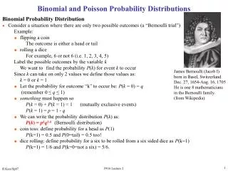
Lecture 2 Binomial and Poisson Probability Distributions. Binomial Probability Distribution l Consider a situation where there are only two possible outcomes (a “Bernoulli trial”) Example: u flipping a coin head or tail u rolling a dice 6 or not 6 (i.e. 1, 2, 3, 4, 5)

E N D
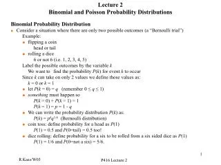
Lecture 2Binomial and Poisson Probability Distributions Binomial Probability Distribution l Consider a situation where there are only two possible outcomes (a “Bernoulli trial”) Example: u flipping a coin head or tail u rolling a dice 6 or not 6 (i.e. 1, 2, 3, 4, 5) Label the possible outcomes by the variable k We want tofind the probability P(k) for event k to occur Since k can take on only 2 values we define those values as: k = 0 or k = 1 u let P(k = 0) = q (remember 0 ≤ q ≤ 1) usomething must happen so P(k = 0) + P(k = 1) = 1 P(k = 1) = p = 1 - q u We can write the probability distribution P(k) as: P(k) = pkq1-k (Bernoulli distribution) u coin toss: define probability for a head as P(1) P(1) = 0.5 and P(0=tail) = 0.5 too! u dice rolling: define probability for a six to be rolled from a six sided dice as P(1) P(1) = 1/6 and P(0=not a six) = 5/6. P416 Lecture 2
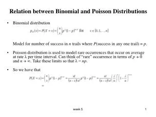
l What is the mean () of P(k)? l What is the Variance (2) of P(k)? l Suppose we have N trials (e.g. we flip a coin N times) what is the probability to get m successes (= heads)? l Consider tossing a coin twice. The possible outcomes are: no heads: P(m = 0) = q2 one head: P(m = 1) = qp + pq (toss 1 is a tail, toss 2 is a head or toss 1 is head, toss 2 is a tail) = 2pq two heads: P(m = 2) = p2 Note: P(m=0)+P(m=1)+P(m=2)=q2+ qp + pq+p2= (p+q)2 = 1 (as it should!) l We want the probability distribution function P(m, N, p) where: m = number of success (e.g. number of heads in a coin toss) N = number of trials (e.g. number of coin tosses) p = probability for a success (e.g. 0.5 for a head) we don't care which of the tosses is a head so there are two outcomes that give one head P416 Lecture 2
l If we look at the three choices for the coin flip example, each term is of the form: CmpmqN-mm = 0, 1, 2, N = 2 for our example, q = 1 - p always! coefficient Cm takes into account the number of ways an outcome can occur without regard to order. for m = 0 or 2 there is only one way for the outcome (both tosses give heads or tails): C0 = C2 = 1 for m = 1 (one head, two tosses) there are two ways that this can occur: C1 = 2. l Binomial coefficients: number of ways of taking N things m at time 0! = 1! = 1, 2! = 1·2 = 2, 3! = 1·2·3 = 6, m! = 1·2·3···m Order of occurrence is not important u e.g. 2 tosses, one head case (m = 1) n we don't care if toss 1 produced the head or if toss 2 produced the head Unordered groups such as our example are called combinations Ordered arrangements are called permutations For N distinguishable objects, if we want to group them m at a time, the number of permutations: u example: If we tossed a coin twice (N = 2), there are two ways for getting one head (m = 1) u example: Suppose we have 3 balls, one white, one red, and one blue. n Number of possible pairs we could have, keeping track of order is 6 (rw, wr, rb, br, wb, bw): n If order is not important (rw = wr), then the binomial formula gives number of “two color” combinations P416 Lecture 2
l Binomial distribution: the probability of m success out of N trials: u p is probability of a success and q = 1 - p is probability of a failure l To show that the binomial distribution is properly normalized, use Binomial Theorem: Þbinomial distribution is properly normalized P416 Lecture 2
l Mean of binomial distribution: A cute way of evaluating the above sum is to take the derivative: l Variance of binomial distribution (obtained using similar trick): P416 Lecture 2
Example: Suppose you observed m special events (success) in a sample of N events u The measured probability (“efficiency”) for a special event to occur is: What is the error on the probability ("error on the efficiency"): The sample size (N) should be as large as possible to reduce certainty in the probability measurement Let’s relate the above result to Lab 2 where we throw darts to measure the value of p. If we inscribe a circle inside a square with side=s then the ratio of the area of the circle to the rectangle is: we will derive this later in the course • So, if we throw darts at random at our rectangle then the probability (ºe) of a dart landing inside the • circle is just the ratio of the two areas, p/4. The we can determine p using: p= 4e. The error in p is related to the error in e by: We can estimate how well we can measure p by this method by assuming that e=p/4= (3.14159…)/4: This formula “says” that to improve our estimate of p by a factor of 10 we have to throw 100 (N) times as many darts! Clearly, this is an inefficient way to determine p. P416 Lecture 2
Example: Suppose a baseball player's batting average is 0.33 (1 for 3 on average). u Consider the case where the player either gets a hit or makes an out (forget about walks here!). prob. for a hit: p = 0.33 prob. for "no hit”: q = 1 - p = 0.67 u On average how many hits does the player get in 100 at bats? = Np = 100·0.33 = 33 hits u What's the standard deviation for the number of hits in 100 at bats? = (Npq)1/2 = (100·0.33·0.67)1/2 ≈ 4.7 hits we expect ≈ 33 ± 5 hits per 100 at bats u Consider a game where the player bats 4 times: probability of 0/4 = (0.67)4 = 20% probability of 1/4 = [4!/(3!1!)](0.33)1(0.67)3 = 40% probability of 2/4 = [4!/(2!2!)](0.33)2(0.67)2 = 29% probability of 3/4 = [4!/(1!3!)](0.33)3(0.67)1 = 10% probability of 4/4 = [4!/(0!4!)](0.33)4(0.67)0 = 1% probability of getting at least one hit = 1 - P(0) = 0.8 P416 Lecture 2
Poisson Probability Distribution l The Poisson distribution is a widely used discrete probability distribution. l Consider the following conditions: p is very small and approaches 0 u example: a 100 sided dice instead of a 6 sided dice, p = 1/100 instead of 1/6 u example: a 1000 sided dice, p = 1/1000 N is very large and approaches ∞ u example: throwing 100 or 1000 dice instead of 2 dice The product Np is finite l Example: radioactive decay Suppose we have 25 mg of an element very large number of atoms: N ≈ 1020 Suppose the lifetime of this element t = 1012 years ≈ 5x10¹⁹ seconds probability of a given nucleus to decay in one second is very small: p = 1/t = 2x10-20/sec Np = 2/sec finite! The number of counts in a time interval is a Poisson process. l Poisson distribution can be derived by taking the appropriate limits of the binomial distribution P416 Lecture 2
um is always an integer ≥ 0 udoes not have to be an integer It is easy to show that: = Np = mean of a Poisson distribution 2 = Np = = variance of a Poisson distribution l Radioactivity example with an average of 2 decays/sec: i) What’s the probability of zero decays in one second? ii) What’s the probability of more than one decay in one second? iii) Estimate the most probable number of decays/sec? u To solve this problem its convenient to maximize lnP(m, ) instead of P(m, ). The mean and variance of a Poisson distribution are the same number! P416 Lecture 2
u In order to handle the factorial when take the derivative we use Stirling's Approximation: The most probable value for m is just the average of the distribution u This is only approximate since Stirlings Approximation is only valid for large m. u Strictly speaking m can only take on integer values while is not restricted to be an integer. If you observed m events in a “counting” experiment, the error on m is ln10!=15.10 10ln10-10=13.03 ®14% ln50!=148.48 50ln50-50=145.60®1.9% P416 Lecture 2
Comparison of Binomial and Poisson distributions with mean m = 1 Not much difference between them! N N For N large and m fixed: Binomial Þ Poisson P416 Lecture 2
What is a uniform probability distribution (p(x))? p(x)=constant (c) for a£x£b p(x)=zero everywhere else Therefore p(x1)dx1= p(x2)dx2 if dx1=dx2Þ equal intervals give equal probabilities For a uniform distribution with a=0, b=1 we have p(x)=1 Uniform distribution and Random Numbers What is a random number generator ? A number picked at random from a uniform distribution with limits [0,1] All major computer languages (FORTRAN, C) come with arandom number generator. FORTRAN: RAN(iseed) The following FORTRAN program generates 5 random numbers: iseed=12345 do I=1,5 y=ran(iseed) type *, y enddo end 0.1985246 0.8978736 0.2382888 0.3679854 0.3817045 If we generate “a lot” of random numbers all equal intervals should contain the same amount of numbers. For example: generate: 106 random numbers expect: 105 numbers [0.0, 0.1] 105 numbers [0.45, 0.55] P416 Lecture 2
When we throw an “honest” 6 sided dice we expect each number to appear 1/6 of the time. To simulate this on the computer we want a program that generates the integers [1, 2, 3, 4, 5, 6] in a way that each number is equally likely. DICE=INT(1+6*RAN(ISEED)) RAN(ISEED) Þgives a number [0,1], e.g. 0.33 6*RAN(ISEED) Þ1.98 1+6*RAN(ISEED) Þ2.98 INT(1+6*RAN(ISEED)) Þtruncates 2.98 to an integer, 2 We just rolled a “2” How would we roll two dice with a computer? DICE1= INT(1+6*RAN(ISEED)) DICE2= INT(1+6*RAN(ISEED)) TWODI=DICE1+DICE2 The variable TWODI is an integer [1,12] which corresponds to the sum of the numbers on two independent rolls of the dice. Throwing a dice using a computer P416 Lecture 2