Download
1 / 38
380 likes | 741 Vues
INTRODUCTION TO RESOURCE SELECTION BY ANIMALS University of Wyoming 11-12 January, 2003 Module 5 Resource Selection Functions by Logistic Regression Presented by Bryan F.J. Manly Western EcoSystems Technology Inc. Module 2 Logistic Regression.

E N D
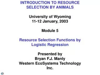
INTRODUCTION TO RESOURCESELECTION BY ANIMALSUniversity of Wyoming11-12 January, 2003Module 5Resource Selection Functions byLogistic RegressionPresented byBryan F.J. ManlyWestern EcoSystems TechnologyInc.
Module 2Logistic Regression One of the simplest ways of estimating aresource selection probability functioninvolves using logistic regression for modelling the probability of use of resourceunits, based on a collection of such units.Logistic regression can also be used withsamples of resource units, although this iscomplicated by the need to vary theestimation procedure according to thesampling protocol that is used.These uses of logistic regression are covered in this module and illustrated using data on the selection of winter habitat by antelopes and nest site selection by fernbirds. Chapter 5 in Resource Selection by Animals:Statistical Design and Analysis for Field Studies,2nd Edit (RSBA2).
Summary • Census data • Use with a random sample of resource units • Antelope example • Separate sampling • Separate samples of available and used resource units • Separate samples of available and unused resource units • Separate samples of used and unused resource units • Fernbird example
Census Data • Suppose N available resource units. • Known which of these have been used and which have not been used after a single period of selection. • Logistic regressioncan be used to relate the probability of use to variables X1 to XP that are measured on the resource units. • Resource selection probability function • (RSPB) is assumed to take the form • where x = (x1,x2,...,xP) holds the values for the X variables that are measured on a unit.
The logistic function has the desirable property of restricting values of w*(x) to the range 0 to 1, but is otherwise arbitrary. • Other functions that could be used include theprobit where (z) is the integral from -to z for the standard normal distribution, and the proportional hazards function • The main justification for using the logistic function rather than any other to approximate the resource selection probability function is the fact that it is widely used for other statistical analyses in biology, and computer programs for estimating the function are readily available.
Suppose that the N available resource units can be divided into I groups so that within the ith group the units have the same values xi = (xi1,xi2,...,xiP) for the X variables. • The number of used resource units in group i, ui, can then be assumed to be a random value from the binomial distribution with parameters Ai and w*(xi), where Ai is the number of available resource units in the group. • Maximum likelihood estimation using any of the standard computer programs for logistic regression. • Often all of the available resource units will have different values for the X variables, giving groups of size 1 - causes no difficulties as far as estimation is concerned.
The deviancecan under certain conditions be used as a statistic indicating the goodness of fit of the model. • The condition for the deviance to have an approximately chi-squared distribution is that most values of Aiw*(x){1 - w*(x)} are 'large', which in practice means that they are five or more. • Differencesbetween the deviances for different models can reliably be tested against the chisquared distribution even when the values of Aiw*(x){1 - w*(x)} are small. • See RSBA2 (p. 84) for details of how to calculate the deviance for the 'no selection' model if necessary.
Use With a Sample of Resource Units • Suppose that the units for which information is available are not all of the resource units in the population. • A random sample of units is selected from the full population and it is observed whether each of these is used or not. • Logistic regression can still be used to approximate the probability of use for the ith unit,and logistic regression can be applied to the sample just as well as if there had been a full census.
If the sampled units come from only a small part of the area covered by the full population then logistic regression can still be used: (a) The population of interest can be redefined to consist only of those in the smaller area. Nothing can then be said about the resource selection function in other areas. (b) It can be assumed that the resource selection function is the same everywhere, and can therefore be estimated by a sample from just a part of the total area. Based on this assumption, the estimated function applies everywhere. • If (b) is assumed then the estimation of a resource selection function does not require that the units analysed are a random sample from the population of interest. • A model-based approach that draws its validity only from the assumption that the logistic regression model is correct.
Example: Habitat Selection by Antelope • Study carried out by Ryder (1983) on winter habitat selection by antelope in the Red Rim area in south-central Wyoming. • Ryder set up 256 study plots and recorded the presence or absence of antelope in the winters of 1980-81 and 1981-82, together with a number of characteristics of each plot. • Study area consists of alternating blocks of public and private land - study plots are a systematic sample of 10% of the public land.
Possibilities in terms of the population of resource units that an estimated resource selection function applies to: (a) The 256 sampled plots can be regarded as the population of interest. (b) It can be assumed that the resource selection function is the same on all public land – the estimated function applies to all plots in this population. (c) It can be assumed that the resource selection function is the same on all public and private land. In that case, the estimated function applies to the whole of the Red Rim area. • A matter of judgement as to which of thesepopulations is relevant. • Assume (b) is appropriate.
The distribution of the distance to water and the use of the East/Northeast aspect seem different for different years/use and non-use. Logistic Regression • To allow the estimation of a resource selection probability function where each of the four aspects (E/NE, S/SE, W/SW and N/NW) has a different probability of use, three 0-1 indicator variables can be used to replace the single aspect number: Ind1 = 1 for an E/NE plot or otherwise 0 Ind2 = 1 for a S/SE plot or otherwise 0 Ind3 = 1 for a W/SW plot or otherwise 0. N/NW aspect treated as the 'standard' aspect,which others differ from.
Nine variables available to characterize each of the 256 study plots: X1 = density (thousands/ha) of big sagebrush X2 = density (thousands/ha) of black greasewood X3 = density (thousands/ha) of Nuttall's saltbush X4 = density (thousands/ha) of Douglas rabbitbrush X5 = slope (degrees) X6 = distance to water(m) X7 = East/Northeast indicator variable X8 = South/Southeast indicator variable X9 = West/Southwest indicator variable
Several approaches that can be used for analysing the data by logistic regression, depending on what definition of 'use' is applied: (a)A study plot can be considered to be 'used' if antelopes are recorded in either the first or the second winter - application of logistic regression to approximate the probability of a plot being used is straightforward. (b) A study plot can be considered to be 'used' if antelopes are recorded in both years -probabilities of 'use' that are smaller than for definition (a), but an analysis of the data using logistic regression is still straightforward. (c) A study plot can be considered to be 'used‘ when antelopes are recorded for the first time - requires that the effect of time be modelled - problems with logistic regression.
(d) The two years can be considered to be replicates - logistic regression can be used separately in each year, or one equation can be fitted to both years of data – more complicated analysis than is needed if one of the definitions (a) and (b) is used but better use is made of the data. • Approach (d) used here. • Observational unit will be taken to be a study plot in one year - 512 units, each of which is recorded as either being used or not used. • Question of whether it is reasonable to regard the two years as providing independent data is considered later.
Three logistic regression models have been fitted to the data. • Model 1: assumed that the resource selection probability function was different for the two winters 1980-81 and 1981-82. From comparing deviances (goodness of fit statistics) some evidence of selection in 1980-81 (and overall) but not in 1981-82.
Model 2: refitted the logistic regression equations, again separately for each year, with the vegetation variables and the slope omitted. • The deviance for model 2 is 289.3 with 251 df for 1980-81 - an increase of 3.0 over the deviance for model 1, with +5 df, which is not at all significantly large. • For 1981-82 the deviance for model 2 is 328.8 with 251 df, an increase of 5.2 over model 1, with 5 df. Again, this is not at all significant. • The difference between the total deviance for model 2 and the null model deviance is 22.7 with 8 df - significantly large at the 1% level, giving strong evidence of selection overall.
Model 3: similar coefficients for the two years suggest that it may be possible to get about as good a result by fitting all the data together with a dummy variable introduced to allow for a difference between the years. • The dummy variable 'Year' was set equal to 0 for all the 1980-81 results and 1 for all the 1981-82 results. • The total deviance for model 2 is 618.1 with 502 df, while the total deviance for model 3 is 621.3 with 506 df -difference is 3.2 with 4 df, which is not at all significant - simpler model 3 seems better for describing the data. • Also best model by AIC.
The estimated resource selection probability function (RSPF) is • See RSBA2 (Example 5.1) for more discussion of model diagnostics, etc.
Separate Sampling • Suppose that independent separate random samples are taken of different types of unit. • Logistic regression can then still be used, but it needs a special justification, which depends on the types of samples involved. • Three situations: (a) there is a sample of the available unitsand a sample of the used unitsin the population, (b) there is a sample of the available unitsand a sample of the unused unitsin the population, and (c) there is a sample of unused unitsand a sample of used units.
Separate Samples of Available and Used UnitsExamples • A random sample is taken of the trees in an area that might be used for nests of a species of bird, and a random sample of trees with nests is taken in the same area.Characteristics of the trees in both samples are measured to determine which of these seems important for the selection of nesting sites by the birds. • The locations of groups of moose is recorded from aerial surveys in a national park, and a sample of available locations is selected from a geographical information system (GIS). The characteristics of the locations in both samples are determined from the GIS, possibly in terms of the pixels where they occur, to see what type of location is selected by the moose.
Assume: the population of available units is of size N and ith unit has values xi = (xi1,xi2,...,xip) for the variables X1 to XP, and a corresponding probability of w*(xi) of being used after a certain amount of time. • Every available unit has a probability Pa of being sampled, and every used unit has a probability Pu of being sampled. Available units sampled first (without replacement). Then • The probability of a unit being used and sampled is (1 - Pa)w*(xi)Pu, and the probability of a unit being in either the available or the used sample is Prob(ith unit sampled) = Pa + (1 - Pa)w*(xi)Pu.
Assume that the RSPF takes the form where the argument of the exponential function should be negative. Then leading to for the probability of use given that a unit is sampled.
A logistic regression equation in which the parameter b0 is modified to loge[(1-Pa)Pu/Pa]+b0 to allow for available and used resource units being sampled with different probabilities. • Can be fitted by a standard logistic regression equation - see RSBA2 (p. 84). • If the Pu and Pa are known then the parameter b0 in the resource selection probability function can be estimated by subtracting loge[(1-Pa)Pu/Pa] from the estimated constant in the logistic regression equation. • Otherwise b0 cannot be estimated, but it is still possible to estimate the RSF w(x) = exp(b1x1 + ... + bPxP) and use this to compare resource units. • Best to use sampling with sampling probabilities of Pa and Pu, but fixed size samples and/or systematic samples are possible.
Need to ensure if possible that no units have probabilities of use over 1by this model, i.e. w*(xi) = exp(b0 +b1xi1 + ... + bPxiP) 1 for all units in the population. • Can be checked if sampling probabilities are known so that b0 can be estimated. • Should be okay if all probabilities of use are obviously quite small.
Separate Samples of Available and Unused Resource UnitsExamples • The prey items available in an area are sampled before and after a predator is introduced, to determine what type of prey the predator chooses. • Plots of land not used by an animal are sampled, and compared with a sample of all plots in the study area. Characteristics of the plots are measured to determine which are related to the probability of use by the animal. • Leads to a different type of modified logistic regression model - seeRSBA2(p. 102).
Separate Samples of Used and Unused Resource UnitsExamples • Samples of the prey items in an area are sampled after predation by animals, and stomach samples are taken of used prey items. These samples are compared to see which types of prey are selected by the animals. • A study area is divided into plots where it is easy to see which plots have been used by animals, but recording information on the plots is a time consuming process. This information is obtained for a sample of the used plots and a separate sample of the unused plots to determine which characteristics of the plots are related to the probability of use. • Again leads to a third type of modified logistic regression model - seeRSBA2(p. 103).
Example: Nest selection by fernbirds • Harris’ (1986) study on nest selection by fernbirds. • A sample of available resource units (random points in the study region) and a sample of used resource units (nest sites). • Sampling fractions are unknown, but are clearly very small.
A logistic regression was carried out, with the dependent variable being 0 for available sites and 1 for nest sites, and the three variables canopy height, distance to edge, and perimeter of clump used as predictor variables. • Produced the fitted equation • Deviance is 40.48 with 45 df, compared to the deviance of 67.91 with 48 df for the no selection model. • Difference in deviances is 27.43 with 3 df – very highly significant in comparison with the chisquared distribution (p < 0.001), giving strong evidence for selection.
Standard errors for the coefficients of CANOPY, EDGE and PERIM are 3.25, 0.12, and 0.48, espectively. • Ratios of the estimated coefficients to their standard errors to test for the significance of these estimates against the standard normal distribution gives: 7.80/3.25 = 2.40 (p = 0.016) for CANOPY 0.21/0.12 = 1.73 (p = 0.083) for EDGE 0.88/0.48 = 1.84 (p = 0.066) for PERIM • Dropping EDGE and PERIM from the model gives a change close to 5% significance - therefore seems reasonable to accept the model as it stands, with all three variables included.
Estimated RSPF would be if the ratio of sampling probabilities Pu/Pa were known. • Because this ratio is not known, all that can be estimated is the resource selection function that is obtained by omitting the terms -10.73 - loge(Pu/Pa) from the last equation, i.e.,
Summary • Census data • Use with a random sample of resource units • Antelope example • Separate sampling • Separate samples of available and used resource units • Separate samples of available and unused resource units • Separate samples of used and unused resource units • Fernbird example