Download
1 / 76
760 likes | 1.28k Vues
Preliminary Results. Mitigating Computer Platform Radio Frequency Interference in Embedded Wireless Transceivers. February 25, 2008. Outline. Problem Definition I: Single Carrier, Single Antenna Communication Systems Noise Modeling Estimation of Noise Model Parameters

E N D
Preliminary Results Mitigating Computer Platform Radio Frequency Interference inEmbedded Wireless Transceivers February 25, 2008
Outline Problem Definition I: Single Carrier, Single Antenna Communication Systems • Noise Modeling • Estimation of Noise Model Parameters • Filtering and Detection • Bounds on Communication Performance II: Single Carrier, Multiple Antenna Communication Systems III: Multiple Carrier, Single Antenna Communication Systems Conclusion and Future Work
Problem Definition • Within computing platforms, wirelesstransceivers experience radio frequencyinterference (RFI) from clocks/busses • Objectives • Develop offline methods to improve communication performance in presence of computer platform RFI • Develop adaptive online algorithms for these methods Approach • Statistical modeling of RFI • Filtering/detection based on estimation of model parameters Backup We’ll be using noise and interference interchangeably
1. Noise Modeling • RFI is combination of independent radiation events, and predominantly has non-Gaussian statistics • Statistical-Physical Models (Middleton Class A, B, C) • Independent of physical conditions (universal) • Sum of independent Gaussian and Poisson interference • Models nonlinear phenomena governing electromagnetic interference • Alpha-Stable Processes • Models statistical properties of “impulsive” noise • Approximation to Middleton Class B noise Backup
[Middleton, 1999] Middleton Class A, B, C Models Class ANarrowband interference (“coherent” reception) Uniquely represented by two parameters Class BBroadband interference (“incoherent” reception) Uniquely represented by six parameters Class CSum of class A and class B (approx. as class B)
Probability Density Function for A = 0.15, G = 0.1 Middleton Class A Model Backup Probability density function (pdf)
Symmetric Alpha Stable Model Characteristic function: Backup Parameters Characteristic exponent indicativeof thickness of tail of impulsiveness Localization (analogous to mean) Dispersion (analogous to variance) No closed-form expression for pdf except for α = 1 (Cauchy), α = 2 (Gaussian), α = 1/2 (Levy) and α = 0 (not very useful) Could approximate pdf using inverse transform of power series expansion of characteristic function Backup
2. Estimation of Noise Model Parameters For the Middleton Class A Model • Expectation maximization (EM) [Zabin & Poor, 1991] • Based on envelope statistics [Middleton, 1979] • Based on moments [Middleton, 1979] For the Symmetric Alpha Stable Model • Based on extreme order statistics [Tsihrintzis & Nikias, 1996] For the Middleton Class B Model • No closed-form estimator exists • Approximate methods based on envelope statistics or moments Backup Backup • Complexity • Iterative algorithm • At each iteration: • Rooting a second order polynomial (Given A, maximize K (= AΓ) ) • Rooting a fourth order polynomial (Given K, maximize A) • Advantage Small sample size required (~1000 samples) • Disadvantage Iterative algorithm, computationally intensive Backup Backup Complexity Parameter estimators are based on simple order statistics AdvantageFast / computationally efficient (non-iterative) Disadvantage Requires large set of data samples (N ~ 10,000) Backup
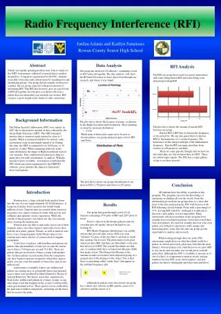
Results on Measured RFI Data Data set of 80,000 samples collected using 20 GSPS scope • Measured data is "broadband" noise • Middleton Class B model would match PDF is symmetric • Symmetric Alpha Stable Process expected to work well • Approximation to Class B model
Results on Measured RFI Data Modeling PDF as Symmetric Alpha Stable process Normalized MSE = 0.0055
Nonlinear Filter Matched Filter v[n] Pulse Shape s[n] gtx[n] grx[n] Λ(.) 3. Filtering and Detection – System Model Alternate Adaptive Model Impulsive Noise Signal Model Multiple samples/copies of the received signal are available: • N path diversity [Miller, 1972] • Oversampling by N[Middleton, 1977] Using multiple samples increases gains vs. Gaussian case because impulses are isolated events over symbol period Backup Decision Rule
Filtering and Detection We assume perfect estimation of noise model parameters Class A Noise • Correlation Receiver (linear) • Wiener Filtering (linear) • Coherent Detection using MAP (Maximum A posteriori Probability) detector[Spaulding & Middleton, 1977] • Small Signal Approximation to MAP Detector[Spaulding & Middleton, 1977] Alpha Stable Noise • Correlation Receiver (linear) • MAP Approximation • Myriad Filtering[Gonzalez & Arce, 2001] • Hole Punching[Ambike et al., 1994] Backup Backup Backup
Coherent Detection – Small Signal Approximation Expand noise pdf pZ(z) by Taylor series about Sj = 0 (j=1,2) Optimal decision rule & threshold detector for approximation Optimal detector for approximation is logarithmic nonlinearity followed by correlation receiver We use 100 terms of the series expansion ford/dxi ln pZ(xi) in simulations Backup
Class A Detection - Results Pulse shapeRaised cosine10 samples per symbol10 symbols per pulse ChannelA = 0.35G = 0.5 × 10⁻³Memoryless K: Constellation Size N: number of samples per symbol M: number of retained terms of the series expansion W: Window Size
Filtering and Detection – Alpha Stable Model MAP detection: remove nonlinear filter Decision rule is given by (p(.) is the SαS distribution) Approximations for SαS distribution:
MAP Detector – PDF Approximation SαS random variable Z with parameters a , d, gcan be written Z = X Y½[Kuruoglu, 1998] • X is zero-mean Gaussian with variance 2 g • Y is positive stable random variable with parameters depending on a Pdf of Z can be written as amixture model of N Gaussians[Kuruoglu, 1998] • Mean d can be added back in • Obtain fY(.) by taking inverse FFT of characteristic function & normalizing • Number of mixtures (N) and values of sampling points (vi) are tunable parameters
Myriad Filtering Sliding window algorithm Outputs myriad of sample window Myriad of order k for samples x1, x2, … , xN [Gonzalez & Arce, 2001] • As k decreases, less impulsive noise gets through myriad filter • As k→0, filter tends to mode filter (output value with highest freq.) Empirical choice of k: [Gonzalez & Arce, 2001]
Myriad Filtering – Implementation Given a window of samples x1,…,xN, find β [xmin, xmax] Optimal myriad algorithm • Differentiate objective functionpolynomial p(β) with respect to β • Find roots and retain real roots • Evaluate p(β) at real roots and extremum • Output β that gives smallest value of p(β) Selection myriad (reduced complexity) • Use x1,…,xN as the possible values of β • Pick value that minimizes objective function p(β) Backup
Hole Punching (Blanking) Filter Sets sample to 0 when sample exceeds threshold [Ambike, 1994] Intuition: • Large values are impulses and true value cannot be recovered • Replace large values with zero will not bias (correlation) receiver • If additive noise were purely Gaussian, then the larger the threshold, the lower the detrimental effect on bit error rate
Complexity Analysis N is oversampling factor S is constellation size W is window size
4. Performance Bounds in presence of impulsive noise Channel Capacity System Model
Capacity in Presence of Impulsive Noise System Model Capacity
Probability of Error for Uncoded Transmission Backup [Haring & Vinck, 2002] BPSK uncoded transmission One sample per symbol A = 0.1, Γ = 10-3
Chernoff Factors for Coded Transmission PEP: Pairwise error probability N: Size of the codeword Chernoff factor: Equally likely transmission for symbols
Part IISingle Carrier, Multiple Antenna Communication Systems
Multiple Input Multiple Output (MIMO) Receivers in Impulsive Noise Statistical Physical Models of Noise • Middleton Class A model for two-antenna systems[MacDonald & Blum,1997] • Extension to larger than 2 2 case is difficult Statistical Models of Noise • Multivariate Alpha Stable Process • Mixture of weighted multivariate complex Gaussians as approximation to multivariate Middleton Class A noise[Blum et al., 1997]
MIMO Receivers in Impulsive Noise Key Prior Work • Performance analysis of standard MIMO receivers in impulsive noise[Li, Wang & Zhou, 2004] • Space-time block coding over MIMO channels with impulsive noise[Gao & Tepedelenlioglu,2007] • Assumes uncorrelated noise at antennas Our Contributions • Performance analysis of standard MIMO receivers using multivariate noise models • Optimal and sub-optimal maximum likelihood (ML) receiver design for 2 2 case
Communication Performance 2 x 2 MIMO system A = 0.1, Γ1 = Γ2 = 10-3 Correlation Coeff. = 0.1 Spatial Multiplexing Mode
Part IIIMultiple Carriers, Single Antenna Communication Systems
Motivation Impulse noise with impulse event followed by “flat” region • Coding and interleaving may improve communication performance • In multicarrier modulation, impulsive event in time domain spreads out over all subsymbols thereby reducing effect of impulse Complex number (CN) codes [Lang, 1963] • Transmitter forms s = GS, where S contains transmitted symbols,G is a unitary matrix and s contains coded symbols • Receiver multiplies received symbols by G-1 • Gaussian noise unaffected (unitary transformation is rotation) • Orthogonal frequency division multiplexing (OFDM) is special case of CN codes when G is inverse discrete Fourier transformmatrix
Noise Smearing Smearing effect • Impulsive noise energy distributes over longer symbol time • Smearing filters maximize impulse attenuation and minimize intersymbol interference for impulsive noise [Beenker, 1985] • Maximum smearing efficiency is where N is number of symbols used in unitary transformation • As N, distribution of impulsive noise becomes Gaussian Simulations [Haring, 2003] • When using a transformation involving N = 1024 symbols, impulsive noise case approaches case where only Gaussian noise is present Backup
Conclusion Radio frequency interference from computing platform • Affects wireless data communication transceivers • Models include Middleton noise models and alpha stable processes • Cancellation can improve communication performance Initial RFI cancellation methods explored • Linear (Wiener) and Non-linear filtering (Myriad, Hole Punching) • Optimal detection rules (significant gains at low bit rates) Preliminary work • Performance bounds in presence of RFI • RFI mitigation in multicarrier, MIMO communication systems
Contributions Publications M. Nassar, K. Gulati, A. K. Sujeeth, N. Aghasadeghi, B. L. Evans and K. R. Tinsley, “Mitigating Near-field Interference in Laptop Embedded Wireless Transceivers”, Proc. IEEE Int. Conf. on Acoustics, Speech, and Signal Proc., Mar. 30-Apr. 4, 2008, Las Vegas, NV USA, accepted for publication. Software Releases RFI Mitigation Toolbox Version 1.1 Beta (Released November 21st, 2007) Version 1.0 (Released September 22nd, 2007) http://users.ece.utexas.edu/~bevans/projects/rfi/software.html Project Web Site http://users.ece.utexas.edu/~bevans/projects/rfi/index.html
Future Work Single carrier, single antenna communication systems • Fixed-point (embedded) methods for parameter estimation and detection methods • Estimation and detection for Middleton Class B model Single carrier, multiple antenna communication systems • MIMO receiver design in presence of RFI • Performance bounds for MIMO receivers in presence of RFI Multicarrier Modulation and Coding • Explore unitary coding schemes resilient to RFI • Investigate multi-layered coding
References [1] D. Middleton, “Non-Gaussian noise models in signal processing for telecommunications: New methods and results for Class A and Class B noise models”, IEEE Trans. Info. Theory, vol. 45, no. 4, pp. 1129-1149, May 1999 [2] S. M. Zabin and H. V. Poor, “Efficient estimation of Class A noise parameters via the EM [Expectation-Maximization] algorithms”, IEEE Trans. Info. Theory, vol. 37, no. 1, pp. 60-72, Jan. 1991 [3] G. A. Tsihrintzis and C. L. Nikias, "Fast estimation of the parameters of alpha-stable impulsive interference", IEEE Trans. Signal Proc., vol. 44, Issue 6, pp. 1492-1503, Jun. 1996 [4] A. Spaulding and D. Middleton, “Optimum Reception in an Impulsive Interference Environment-Part I: Coherent Detection”, IEEE Trans. Comm., vol. 25, no. 9, Sep. 1977 [5] A. Spaulding and D. Middleton, “Optimum Reception in an Impulsive Interference Environment-Part II: Incoherent Detection”, IEEE Trans. Comm., vol. 25, no. 9, Sep. 1977 [6] B. Widrow et al., “Principles and Applications”, Proc. of the IEEE, vol. 63, no.12, Sep. 1975. [7] J.G. Gonzalez and G.R. Arce, “Optimality of the Myriad Filter in Practical Impulsive-Noise Environments”, IEEE Trans. on Signal Processing, vol 49, no. 2, Feb 2001
References (cont…) [8] S. Ambike, J. Ilow, and D. Hatzinakos, “Detection for binary transmission in a mixture of gaussian noise and impulsive noise modeled as an alpha-stable process,” IEEE Signal Processing Letters, vol. 1, pp. 55–57, Mar. 1994. [9] J. G. Gonzalez and G. R. Arce, “Optimality of the myriad filter in practical impulsive-noise enviroments,” IEEE Trans. on Signal Proc, vol. 49, no. 2, pp. 438–441, Feb 2001. [10] E. Kuruoglu, “Signal Processing In Alpha Stable Environments: A Least Lp Approach,” Ph.D. dissertation, University of Cambridge, 1998. [11] J. Haring and A.J. Han Vick, “Iterative Decoding of Codes Over Complex Numbers for Impuslive Noise Channels”, IEEE Trans. On Info. Theory, vol 49, no. 5, May 2003 [12] G. Beenker, T. Claasen, and P. van Gerwen, “Design of smearing filters for data transmission systems,” IEEE Trans. on Comm., vol. 33, Sept. 1985. [13] G. R. Lang, “Rotational transformation of signals,” IEEE Trans. Inform. Theory, vol. IT–9, pp. 191–198, July 1963. [14] Ping Gao and C. Tepedelenlioglu. “Space-time coding over mimo channels with impulsive noise”, IEEE Trans. on Wireless Comm., 6(1):220–229, January 2007. [15] K.F. McDonald and R.S. Blum. “A physically-based impulsive noise model for array observations”, Proc. IEEE Asilomar Conference on Signals, Systems& Computers, vol 1, 2-5 Nov. 1997.
Potential Impact Improve communication performance for wireless data communication subsystems embedded in PCs and laptops • Achieve higher bit rates for the same bit error rate and range, and lower bit error rates for the same bit rate and range • Extend range from wireless data communication subsystems to wireless access point Extend results to multipleRF sources on single chip
Accuracy of Middleton Noise Models Magnetic Field Strength, H (dB relative to microamp per meter rms) ε0 (dB > εrms) Percentage of Time Ordinate is Exceeded P(ε > ε0) Soviet high power over-the-horizon radar interference [Middleton, 1999] Fluorescent lights in mine shop office interference [Middleton, 1999]
Middleton Class A Statistics Envelope statistics Envelope for Gaussian signal has Rayleigh distribution Power Spectral Density
Symmetric Alpha Stable Process PDF Closed-form expression does not exist in general Power series expansions can be derived in some cases Standard symmetric alpha stable model for localization parameter d = 0
Symmetric Alpha Stable Statistics Example: exponent a = 1.5, “mean” d = 0and “variance” g = 10 ×10-4 Probability Density Function Power Spectral Density
Estimation of Middleton Class A Model Parameters Expectation maximization • E: Calculate log-likelihood function w/ current parameter values • M: Find parameter set that maximizes log-likelihood function EM estimator for Class A parameters[Zabin & Poor, 1991] • Expresses envelope statistics as sum of weighted pdfs Maximization step is iterative • Given A, maximize K (with K = AΓ). Root 2nd-order polynomial. • Given K, maximize A. Root4th-order poly. (after approximation). Backup Backup
Estimation of Symmetric Alpha Stable Parameters Based on extreme order statistics [Tsihrintzis & Nikias, 1996] PDFs of max and min of sequence of independently and identically distributed (IID) data samples follow • PDF of maximum: • PDF of minimum: Extreme order statistics of Symmetric Alpha Stable pdf approach Frechet’s distribution as N goes to infinity Parameter estimators then based on simple order statistics • AdvantageFast / computationally efficient (non-iterative) • Disadvantage Requires large set of data samples (N ~ 10,000) Backup Backup Backup
Class A Parameter Estimation Based on APD (Exceedance Probability Density) Plot
e2 = e4 = e6 = Class A Parameter Estimation Based on Moments Moments (as derived from the characteristic equation) Parameter estimates Odd-order momentsare zero[Middleton, 1999] 2
Middleton Class B Model Envelope Statistics Envelope exceedance probability density (APD) which is 1 – cumulative distribution function