Download
1 / 105
1.12k likes | 1.35k Vues
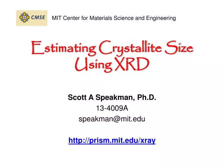
MIT Center for Materials Science and Engineering. Estimating Crystallite Size Using XRD. Scott A Speakman, Ph.D. 13-4009A speakman@mit.edu http://prism.mit.edu/xray. Warning. These slides have not been extensively proof-read, and therefore may contain errors.

E N D
MIT Center for Materials Science and Engineering Estimating Crystallite SizeUsing XRD Scott A Speakman, Ph.D. 13-4009A speakman@mit.edu http://prism.mit.edu/xray
Warning • These slides have not been extensively proof-read, and therefore may contain errors. • While I have tried to cite all references, I may have missed some– these slides were prepared for an informal lecture and not for publication. • If you note a mistake or a missing citation, please let me know and I will correct it. • I hope to add commentary in the notes section of these slides, offering additional details. However, these notes are incomplete so far. http://prism.mit.edu/xray
Goals of Today’s Lecture • Provide a quick overview of the theory behind peak profile analysis • Discuss practical considerations for analysis • Demonstrate the use of lab software for analysis • empirical peak fitting using MDI Jade • Rietveld refinement using HighScore Plus • Discuss other software for peak profile analysis • Briefly mention other peak profile analysis methods • Warren Averbach Variance method • Mixed peak profiling • whole pattern • Discuss other ways to evaluate crystallite size • Assumptions: you understand the basics of crystallography, X-ray diffraction, and the operation of a Bragg-Brentano diffractometer http://prism.mit.edu/xray
A Brief History of XRD • 1895- Röntgen publishes the discovery of X-rays • 1912- Laue observes diffraction of X-rays from a crystal • when did Scherrer use X-rays to estimate the crystallite size of nanophase materials? http://prism.mit.edu/xray
The Scherrer Equation was published in 1918 • Peak width (B) is inversely proportional to crystallite size (L) • P. Scherrer, “Bestimmung der Grösse und der inneren Struktur von Kolloidteilchen mittels Röntgenstrahlen,” Nachr. Ges. Wiss. Göttingen26 (1918) pp 98-100. • J.I. Langford and A.J.C. Wilson, “Scherrer after Sixty Years: A Survey and Some New Results in the Determination of Crystallite Size,” J. Appl. Cryst.11 (1978) pp 102-113. http://prism.mit.edu/xray
The Laue Equations describe the intensity of a diffracted peak from a single parallelopipeden crystal • N1, N2, and N3 are the number of unit cells along the a1, a2, and a3 directions • When N is small, the diffraction peaks become broader • The peak area remains constant independent of N http://prism.mit.edu/xray
Intensity (a.u.) 66 67 68 69 70 71 72 73 74 2 q (deg.) Which of these diffraction patterns comes from a nanocrystalline material? • These diffraction patterns were produced from the exact same sample • Two different diffractometers, with different optical configurations, were used • The apparent peak broadening is due solely to the instrumentation http://prism.mit.edu/xray
Many factors may contribute tothe observed peak profile • Instrumental Peak Profile • Crystallite Size • Microstrain • Non-uniform Lattice Distortions • Faulting • Dislocations • Antiphase Domain Boundaries • Grain Surface Relaxation • Solid Solution Inhomogeneity • Temperature Factors • The peak profile is a convolution of the profiles from all of these contributions http://prism.mit.edu/xray
Instrument and Sample Contributions to the Peak Profile must be Deconvoluted • In order to analyze crystallite size, we must deconvolute: • Instrumental Broadening FW(I) • also referred to as the Instrumental Profile, Instrumental FWHM Curve, Instrumental Peak Profile • Specimen Broadening FW(S) • also referred to as the Sample Profile, Specimen Profile • We must then separate the different contributions to specimen broadening • Crystallite size and microstrain broadening of diffraction peaks http://prism.mit.edu/xray
Contributions to Peak Profile • Peak broadening due to crystallite size • Peak broadening due to the instrumental profile • Which instrument to use for nanophase analysis • Peak broadening due to microstrain • the different types of microstrain • Peak broadening due to solid solution inhomogeneity and due to temperature factors http://prism.mit.edu/xray
Crystallite Size Broadening • Peak Width due to crystallite size varies inversely with crystallite size • as the crystallite size gets smaller, the peak gets broader • The peak width varies with 2q as cos q • The crystallite size broadening is most pronounced at large angles 2Theta • However, the instrumental profile width and microstrain broadening are also largest at large angles 2theta • peak intensity is usually weakest at larger angles 2theta • If using a single peak, often get better results from using diffraction peaks between 30 and 50 deg 2theta • below 30deg 2theta, peak asymmetry compromises profile analysis http://prism.mit.edu/xray
The Scherrer Constant, K • The constant of proportionality, K (the Scherrer constant) depends on the how the width is determined, the shape of the crystal, and the size distribution • the most common values for K are: • 0.94 for FWHM of spherical crystals with cubic symmetry • 0.89 for integral breadth of spherical crystals w/ cubic symmetry • 1, because 0.94 and 0.89 both round up to 1 • K actually varies from 0.62 to 2.08 • For an excellent discussion of K, refer to JI Langford and AJC Wilson, “Scherrer after sixty years: A survey and some new results in the determination of crystallite size,” J. Appl. Cryst.11 (1978) p102-113. http://prism.mit.edu/xray
Factors that affect K and crystallite size analysis • how the peak width is defined • how crystallite size is defined • the shape of the crystal • the size distribution http://prism.mit.edu/xray
Intensity (a.u.) 46.7 46.8 46.9 47.0 47.1 47.2 47.3 47.4 47.5 47.6 47.7 47.8 47.9 2 q (deg.) Intensity (a.u.) 46.7 46.8 46.9 47.0 47.1 47.2 47.3 47.4 47.5 47.6 47.7 47.8 47.9 2 q (deg.) Methods used in Jade to Define Peak Width • Full Width at Half Maximum (FWHM) • the width of the diffraction peak, in radians, at a height half-way between background and the peak maximum • Integral Breadth • the total area under the peak divided by the peak height • the width of a rectangle having the same area and the same height as the peak • requires very careful evaluation of the tails of the peak and the background FWHM http://prism.mit.edu/xray
Integral Breadth • Warren suggests that the Stokes and Wilson method of using integral breadths gives an evaluation that is independent of the distribution in size and shape • L is a volume average of the crystal thickness in the direction normal to the reflecting planes • The Scherrer constant K can be assumed to be 1 • Langford and Wilson suggest that even when using the integral breadth, there is a Scherrer constant K that varies with the shape of the crystallites http://prism.mit.edu/xray
Other methods used to determine peak width • These methods are used in more the variance methods, such as Warren-Averbach analysis • Most often used for dislocation and defect density analysis of metals • Can also be used to determine the crystallite size distribution • Requires no overlap between neighboring diffraction peaks • Variance-slope • the slope of the variance of the line profile as a function of the range of integration • Variance-intercept • negative initial slope of the Fourier transform of the normalized line profile http://prism.mit.edu/xray
How is Crystallite Size Defined • Usually taken as the cube root of the volume of a crystallite • assumes that all crystallites have the same size and shape • For a distribution of sizes, the mean size can be defined as • the mean value of the cube roots of the individual crystallite volumes • the cube root of the mean value of the volumes of the individual crystallites • Scherrer method (using FWHM) gives the ratio of the root-mean-fourth-power to the root-mean-square value of the thickness • Stokes and Wilson method (using integral breadth) determines the volume average of the thickness of the crystallites measured perpendicular to the reflecting plane • The variance methods give the ratio of the total volume of the crystallites to the total area of their projection on a plane parallel to the reflecting planes http://prism.mit.edu/xray
Remember, Crystallite Size is Different than Particle Size • A particle may be made up of several different crystallites • Crystallite size often matches grain size, but there are exceptions http://prism.mit.edu/xray
Crystallite Shape • Though the shape of crystallites is usually irregular, we can often approximate them as: • sphere, cube, tetrahedra, or octahedra • parallelepipeds such as needles or plates • prisms or cylinders • Most applications of Scherrer analysis assume spherical crystallite shapes • If we know the average crystallite shape from another analysis, we can select the proper value for the Scherrer constant K • Anistropic peak shapes can be identified by anistropic peak broadening • if the dimensions of a crystallite are 2x * 2y * 200z, then (h00) and (0k0) peaks will be more broadened then (00l) peaks. http://prism.mit.edu/xray
Anistropic Size Broadening • The broadening of a single diffraction peak is the product of the crystallite dimensions in the direction perpendicular to the planes that produced the diffraction peak. http://prism.mit.edu/xray
Crystallite Size Distribution • is the crystallite size narrowly or broadly distributed? • is the crystallite size unimodal? • XRD is poorly designed to facilitate the analysis of crystallites with a broad or multimodal size distribution • Variance methods, such as Warren-Averbach, can be used to quantify a unimodal size distribution • Otherwise, we try to accommodate the size distribution in the Scherrer constant • Using integral breadth instead of FWHM may reduce the effect of crystallite size distribution on the Scherrer constant K and therefore the crystallite size analysis http://prism.mit.edu/xray
Intensity (a.u.) 47.0 47.2 47.4 47.6 47.8 2 q (deg.) Instrumental Peak Profile • A large crystallite size, defect-free powder specimen will still produce diffraction peaks with a finite width • The peak widths from the instrument peak profile are a convolution of: • X-ray Source Profile • Wavelength widths of Ka1 and Ka2 lines • Size of the X-ray source • Superposition of Ka1 and Ka2 peaks • Goniometer Optics • Divergence and Receiving Slit widths • Imperfect focusing • Beam size • Penetration into the sample Patterns collected from the same sample with different instruments and configurations at MIT http://prism.mit.edu/xray
What Instrument to Use? • The instrumental profile determines the upper limit of crystallite size that can be evaluated • if the Instrumental peak width is much larger than the broadening due to crystallite size, then we cannot accurately determine crystallite size • For analyzing larger nanocrystallites, it is important to use the instrument with the smallest instrumental peak width • Very small nanocrystallites produce weak signals • the specimen broadening will be significantly larger than the instrumental broadening • the signal:noise ratio is more important than the instrumental profile http://prism.mit.edu/xray
Comparison of Peak Widths at 47° 2q for Instruments and Crystallite Sizes • Rigaku XRPD is better for very small nanocrystallites, <80 nm (upper limit 100 nm) • PANalytical X’Pert Pro is better for larger nanocrystallites, <150 nm http://prism.mit.edu/xray
Other Instrumental Considerations for Thin Films • The irradiated area greatly affects the intensity of high angle diffraction peaks • GIXD or variable divergence slits on the PANalytical X’Pert Pro will maintain a constant irradiated area, increasing the signal for high angle diffraction peaks • both methods increase the instrumental FWHM • Bragg-Brentano geometry only probes crystallite dimensions through the thickness of the film • in order to probe lateral (in-plane) crystallite sizes, need to collect diffraction patterns at different tilts • this requires the use of parallel-beam optics on the PANalytical X’Pert Pro, which have very large FWHM and poor signal:noise ratios http://prism.mit.edu/xray
Microstrain Broadening • lattice strains from displacements of the unit cells about their normal positions • often produced by dislocations, domain boundaries, surfaces etc. • microstrains are very common in nanocrystalline materials • the peak broadening due to microstrain will vary as: compare to peak broadening due to crystallite size: http://prism.mit.edu/xray
Contributions to Microstrain Broadening • Non-uniform Lattice Distortions • Dislocations • Antiphase Domain Boundaries • Grain Surface Relaxation • Other contributions to broadening • faulting • solid solution inhomogeneity • temperature factors http://prism.mit.edu/xray
| | | | | | | | | Intensity (a.u.) 26.5 27.0 27.5 28.0 28.5 29.0 29.5 30.0 2 q (deg.) Non-Uniform Lattice Distortions • Rather than a single d-spacing, the crystallographic plane has a distribution of d-spaces • This produces a broader observed diffraction peak • Such distortions can be introduced by: • surface tension of nanocrystals • morphology of crystal shape, such as nanotubes • interstitial impurities http://prism.mit.edu/xray
Antiphase Domain Boundaries • Formed during the ordering of a material that goes through an order-disorder transformation • The fundamental peaks are not affected • the superstructure peaks are broadened • the broadening of superstructure peaks varies with hkl http://prism.mit.edu/xray
Dislocations • Line broadening due to dislocations has a strong hkl dependence • The profile is Lorentzian • Can try to analyze by separating the Lorentzian and Gaussian components of the peak profile • Can also determine using the Warren-Averbach method • measure several orders of a peak • 001, 002, 003, 004, … • 110, 220, 330, 440, … • The Fourier coefficient of the sample broadening will contain • an order independent term due to size broadening • an order dependent term due to strain http://prism.mit.edu/xray
Faulting • Broadening due to deformation faulting and twin faulting will convolute with the particle size Fourier coefficient • The particle size coefficient determined by Warren-Averbach analysis actually contains contributions from the crystallite size and faulting • the fault contribution is hkl dependent, while the size contribution should be hkl independent (assuming isotropic crystallite shape) • the faulting contribution varies as a function of hkl dependent on the crystal structure of the material (fcc vs bcc vs hcp) • See Warren, 1969, for methods to separate the contributions from deformation and twin faulting http://prism.mit.edu/xray
ZrO2 46nm CeO2 19 nm CexZr1-xO2 0<x<1 Intensity (a.u.) 45 46 47 48 49 50 51 52 2 q (deg.) Solid Solution Inhomogeneity • Variation in the composition of a solid solution can create a distribution of d-spacing for a crystallographic plane • Similar to the d-spacing distribution created from microstrain due to non-uniform lattice distortions http://prism.mit.edu/xray
Temperature Factor • The Debye-Waller temperature factor describes the oscillation of an atom around its average position in the crystal structure • The thermal agitation results in intensity from the peak maxima being redistributed into the peak tails • it does not broaden the FWHM of the diffraction peak, but it does broaden the integral breadth of the diffraction peak • The temperature factor increases with 2Theta • The temperature factor must be convoluted with the structure factor for each peak • different atoms in the crystal may have different temperature factors • each peak contains a different contribution from the atoms in the crystal http://prism.mit.edu/xray
Determining the Sample Broadening due to crystallite size • The sample profile FW(S) can be deconvoluted from the instrumental profile FW(I) either numerically or by Fourier transform • In Jade size and strain analysis • you individually profile fit every diffraction peak • deconvolute FW(I) from the peak profile functions to isolate FW(S) • execute analyses on the peak profile functions rather than on the raw data • Jade can also use iterative folding to deconvolute FW(I) from the entire observed diffraction pattern • this produces an entire diffraction pattern without an instrumental contribution to peak widths • this does not require fitting of individual diffraction peaks • folding increases the noise in the observed diffraction pattern • Warren Averbach analyses operate on the Fourier transform of the diffraction peak • take Fourier transform of peak profile functions or of raw data http://prism.mit.edu/xray
Analysis using MDI Jade • The data analysis package Jade is designed to use empirical peak profile fitting to estimate crystallite size and/or microstrain • Three Primary Components • Profile Fitting Techniques • Instrumental FWHM Curve • Size & Strain Analysis • Scherrer method • Williamson-Hall method http://prism.mit.edu/xray
Important Chapters in Jade Help • Jade’s User Interface • User Preferences Dialog • Advanced Pattern Processing • Profile Fitting and Peak Decomposition • Crystallite Size & Strain Analysis http://prism.mit.edu/xray
Intensity (a.u.) 28.5 29.0 29.5 30.0 2 q (deg.) Profile Fitting • Empirically fit experimental data with a series of equations • fit the diffraction peak using the profile function • fit background, usually as a linear segment • this helps to separate intensity in peak tails from background • To extract information, operate explicitly on the equation rather than numerically on the raw data • Profile fitting produces precise peak positions, widths, heights, and areas with statistically valid estimates http://prism.mit.edu/xray
Profile Functions • Diffraction peaks are usually the convolution of Gaussian and Lorentzian components • Some techniques try to deconvolute the Gaussian and Lorentzian contributions to each diffraction peak; this is very difficult • More typically, data are fit with a profile function that is a pseudo-Voigt or Pearson VII curve • pseudo-Voigt is a linear combination of Gaussian and Lorentzian components • a true Voigt curve is a convolution of the Gaussian and Lorentzian components; this is more difficult to implement computationally • Pearson VII is an exponential mixing of Gaussian and Lorentzian components • SA Howard and KD Preston, “Profile Fitting of Powder Diffraction Patterns,”, Reviews in Mineralogy vol 20: Modern Powder Diffraction, Mineralogical Society of America, Washington DC, 1989. http://prism.mit.edu/xray
Important Tips for Profile Fitting • Do not process the data before profile fitting • do not smooth the data • do not fit and remove the background • do not strip Ka2 peaks • Load the appropriate PDF reference patterns for your phases of interest • Zoom in so that as few peaks as possible, plus some background, is visible • Fit as few peaks simultaneously as possible • preferably fit only 1 peak at a time • Constrain variables when necessary to enhance the stability of the refinement http://prism.mit.edu/xray
To Access the Profile Fitting Dialogue Window • Menu: Analyze > Fit Peak Profile • Right-click Fit Profiles button • Right-click Profile Edit Cursor button http://prism.mit.edu/xray
open Ge103.xrdml • overlay PDF reference pattern 04-0545 • Demonstrate profile fitting of the 5 diffraction peaks • fit one at a time • fit using ‘All’ option http://prism.mit.edu/xray
Important Options in Profile Fitting Window 1 2 4 3 5 8 6 7 9 http://prism.mit.edu/xray
1. Profile Shape Function • select the equation that will be used to fit diffraction peaks • Gaussian: • more appropriate for fitting peaks with a rounder top • strain distribution tends to broaden the peak as a Gaussian • Lorentzian: • more appropriate for fitting peaks with a sharper top • size distribution tends to broaden the peak as a Lorentzian • dislocations also create a Lorentzian component to the peak broadening • The instrumental profile and peak shape are often a combination of Gaussian and Lorentzian contributions • pseudo-Voigt: • emphasizes Guassian contribution • preferred when strain broadening dominates • Pearson VII: • emphasize Lorentzian contribution • preferred when size broadening dominates http://prism.mit.edu/xray
2. Shape Parameter • This option allows you to constrain or refine the shape parameter • the shape parameter determines the relative contributions of Gaussian and Lorentzian type behavior to the profile function • shape parameter is different for pseudo-Voigt and Pearson VII functions • pseudo-Voigt: sets the Lorentzian coefficient • Pearson VII: set the exponent • Check the box if you want to constrain the shape parameter to a value • input the value that you want for the shape parameter in the numerical field • Do not check the box if you want the mixing parameter to be refined during profile fitting • this is the much more common setting for this option http://prism.mit.edu/xray
Intensity (a.u.) 25.8 26.0 26.2 26.4 26.6 26.8 27.0 2 q (deg.) 3. Skewness • Skewness is used to model asymmetry in the diffraction peak • Most significant at low values of 2q • Unchecked: skewness will be refined during profile fitting • Checked: skewness will be constrained to the value indicated • usually check this option to constrain skewness to 0 • skewness=0 indicates a symmetrical peak • Hint: constrain skewness to zero when • refining very broad peaks • refining very weak peaks • refining several heavily overlapping peaks an example of the error created when fitting low angle asymmetric data with a skewness=0 profile http://prism.mit.edu/xray
00-027-1402> Silicon - Si Intensity (a.u.) 87.5 88.0 88.5 89.0 2 q (deg.) 4. K-alpha2 contribution • Checking this box indicates that Ka2 radiation is present and should be included in the peak profile model • this should almost always be checked when analyzing your data • It is much more accurate to model Ka2 than it is to numerically strip the Ka2 contribution from the experimental data This is a single diffraction peak, featuring the Ka1 and Ka2 doublet http://prism.mit.edu/xray
Intensity (a.u.) 52 53 54 55 56 57 58 59 60 61 62 63 64 2 q (deg.) 5. Background function • Specifies how the background underneath the peak will be modeled • usually use “Linear Background” • “Level Background” is appropriate if the background is indeed fairly level and the broadness of the peak causes the linear background function to fit improperly • manually fit the background (Analyze > Fit Background) and use “Fixed Background” for very complicated patterns • more complex background functions will usually fail when fitting nanocrystalline materials This linear background fit modeled the background too low. A level fit would not work, so the fixed background must be used. http://prism.mit.edu/xray
Intensity (a.u.) 52 53 54 55 56 57 58 59 60 61 62 63 64 2 q (deg.) 6. Initial Peak Width7. Initial Peak Location • These setting determine the way that Jade calculates the initial peak profile, before refinement • Initial Width • if the peak is not significantly broadened by size or strain, then use the FWHM curve • if the peak is significantly broadened, you might have more success if you Specify a starting FWHM • Initial Location • using PDF overlays is always the preferred option • if no PDF reference card is available, and the peak is significantly broadened, then you will want to manually insert peaks- the Peak Search will not work Result of auto insertion using peak search and FWHM curve on a nanocrystalline broadened peak. Manual peak insertion should be used instead. http://prism.mit.edu/xray
8. Display Options • Check the options for what visual components you want displayed during the profile fitting • Typically use: • Overall Profile • Individual Profiles • Background Curve • Line Marker • Sometimes use: • Difference Pattern • Paint Individuals http://prism.mit.edu/xray
9. Fitting Results • This area displays the results for profile fit peaks • Numbers in () are estimated standard deviations (ESD) • if the ESD is marked with (?), then that peak profile function has not yet been refined • Click once on a row, and the Main Display Area of Jade will move to show you that peak, and a blinking cursor will highlight that peak • You can sort the peak fits by any column by clicking on the column header http://prism.mit.edu/xray