Download
1 / 13
130 likes | 337 Vues
IEG5300 Tutorial 7 Brownian Motion. Peter Chen Peng. Outline. Normal Distribution CLT and statistical estimation Brownian Motion Properties of BM Summary. Normal Distribution. Standard Normal Distribution EX = 0, Var(X) = 1 Rescaling: X -> X+ m EX = m , Var(X) = 2

E N D
IEG5300Tutorial 7Brownian Motion Peter Chen Peng
Outline • Normal Distribution • CLT and statistical estimation • Brownian Motion • Properties of BM • Summary
Normal Distribution • Standard Normal Distribution • EX = 0, Var(X) = 1 • Rescaling: X -> X+m • EX = m, Var(X) = 2 • Called Normal(m, 2) distribution. Note: • E[nX] = nm E[X1+X2+ ... +Xn] = nm • Var(nX) = n22 Var(X1+X2+ ... +Xn) = n2 f(x) 0.6826
Exercise If X and Y are independent identically distributed standard normal random variables, compute Pr{−1 ≤ X + Y ≤ 3}. Solution: X + Y has normal distribution with mean zero and variance 2. So, P[−1 ≤ X + Y ≤ 3] = P[−1/√2 ≤ N(0,1) ≤ 3/√2] = 0.73
CLT Central Limit Theorem (CLT). The standardized sum of i.i.d. X1 = X, X2, ... , Xn is asymptotically of the standard normal distribution. Write EX = m and Var(X) = 2. Then, for all b. Every distribution, when repeated many times, becomes approximately normal. In other words, the sum of any i.i.d. is asymptotically normal. Proven by Fourier transform When n ∞ Binomial(n, m)after standardization :(X1+X2+...+Xn nm)/ normal While Binomial(n, /n) Poisson()
Statistical Estimation • Statistical prediction: • The distribution is known. The target is to predict the next value while minimizing the expected error. • Solution: Optimal predicted value c = EX. The expected error is Var(X). • Statistical Estimation: • Distribution unknown. The target is to estimate EX. • Solution: Optimal EX = (X1+X2+...+Xn )/n. However, the estimation error can be more complexed.
Statistical Estimation • Three parameters are involved: • The sampling size n. • The error tolerance of Y/nm // Or of Y nm. • The confidence level , which is equivalent to b. • Since σ is already known, among the three elements n, b, and , any two among them determine the third.
Brownian Motion Weiner’s Definition. A continuous-time stochastic process {X(t), t≥0} is called a Brownian motion (BM), or sometimes a Wiener process, if : (i) Continuity: (ii) {X(t), t≥0} has stationary independent increments: (a) Independence: is independent of for all (b) Stationarity: The distribution of does not depend on t ; (iii) Normally distributed increments: For • The BM is standard if • X(0) = 0 • = 0 and = 1 where are constant real numbers.
Exercise Suppose that {X(t) : t ≥ 0} is a Brownian motion process with variance parameter σ^2 = 4. Find: P{X(3) ≤ 1|X(2) = 1/2} We have that {B(t) : t ≥ 0} is a standard Brownian motion, where B(t) = X(t)/2. So, P{X(3) ≤ 1|X(2) = 1/2} = P{B(3) ≤1/2|B(2) = 1/4} = P{B(3) − B(2) ≤1/4|B(2) = 1/4} = P{B(3) − B(2) ≤1/4} = P{Z ≤ 0.25} = 0.5987063 Qiwen Wang, IERG4140 Tutorial 8
Brownian Motion • The Normal(0, t) distribution function is • Corollary. The family {Ft}t0of zero-mean distribution functions satisfies • Fs+t = Fs Ft Property 4. Covariance: Property 5 (Scaling invariance). Suppose {X(t)}t ≥ 0is a drift-free BM and a > 0. Then, the process{X *(t)}t ≥ 0defined by is also a standard BM. rescaling a drift-free BM while keeping unchanged -> get the same BM Self-similarity. A part of it (after rescaling) is the same as the whole.
Brownian Motion Property 6. Time-inversion invariance: Let {X(t)}t≥0be a standard BM. Then, so is the following process{X *(t)}t≥0 defined via Property 7: Law of large numbers: Almost surely Notation. The upper and lower right derivatives of a function f are defined as Property 8. Fix t ≥ 0, BM is almost surely not differentiable at t. // In short, X(t) is nowhere differentiable. Moreover,
Summary • Normal(m, 2) distribution: • CLT: • Brownian Motion: • Scaling invariance: Suppose {X(t)}t ≥ 0is a drift-free BM and a > 0. Then, the process{X *(t)}t ≥ 0defined by is also a standard BM.
Extra: Facts about BM • Almost surely, B(t) is nowhere differentiable • Almost surely, B(t) is not monotonic on any interval. • Almost surely, B(t) has infinitely many zeros in every time interval (0, ε), where ε > 0. • On any two fixed intervals, B(t) almost surely does not attain the same maximum. • ……