Download
1 / 53
530 likes | 690 Vues
Model Parameterizations: Issues important for heavy rainfall forecasting. Mike Baldwin NSSL SPC CIMMS. Skill of current operational models. To put it kindly… Current NCEP models do a poor job forecasting heavy rainfall AVN (red), Eta (green), NGM (blue) for Jan-Sept 2000.

E N D
Model Parameterizations: Issues important for heavy rainfall forecasting Mike Baldwin NSSL SPC CIMMS
Skill of current operational models • To put it kindly… • Current NCEP models do a poor job forecasting heavy rainfall • AVN (red), Eta (green), NGM (blue) for Jan-Sept 2000
Ingredients needed by a model in order to predict some phenomena of interest • Adequate grid spacing • To be able to resolve the feature • Physical processes • All those important in the development, maintenance, and decay of the feature • Dynamics • Accuracy, hydrostatic/non-hydrostatic • Adequate initial/boundary conditions • To be able to capture important forcing
Ask yourself: • “Does the model I’m using have the necessary ingredients to predict the feature(s) that I’m considering or expecting?” YES: model guidance taken literally can be useful NO: model by itself is of little value (but not worthless) Either way: knowledge of model characteristics will increase the value of NWP guidance
What are Model Parameterizations? • Techniques used in NWP to predict the collective effects of physical processes which cannot be explicitly resolved • Sub-grid scale or perhaps near-grid scale processes: • For example; cloud physics, convection, turbulent mixing, radiation, surface exchanges
Interaction between different processes is critical • Especially for mesoscale models • Not only important to do a good job with a specific physical process • All pieces have to work well together in order for model to perform well • Several studies have shown great forecast sensitivity to subtle changes to a parameterization
Outline • Quick overview of convective parameterizations currently available in NWP models (both operational and research) • Look at some research/case studies of NWP performance in heavy rain events • Talk about future
Current EMC models use different approaches • RUC II: Grell scheme • Eta: Betts-Miller-Janjic (Kain-Fritsch used experimentally at NSSL & SPC) • MRF/AVN: Grell-Pan scheme • Grell, Grell-Pan, and Kain-Fritsch schemes are Mass-Fluxschemes, meaning they use simple cloud models to simulate rearrangements of mass in a vertical column • Betts-Miller-Janjic adjusts to “mean post-convective profiles” based on observational studies
MM5 Model Physics Options • Precipitation physics • Cumulus parameterization schemes: • Anthes-Kuo • Grell • Kain-Fritsch • Fritsch-Chappell • Betts-Miller • Arakawa-Schubert • Resolvable-scale microphysics schemes: • Removal of supersaturation • Hsie's warm rain scheme • Dudhia's simple ice scheme • Reisner's mixed-phase scheme • Reisner's mixed-phase scheme with graupel • NASA/Goddard microphysics with hail/graupel • Schultz mixed-phase scheme with graupel
MM5 Model Physics Options • Planetary boundary layer parameterization • Bulk formula • Blackadar scheme • Burk-Thompson (Mellor-Yamada 1.5-order/level-2.5 scheme) • Eta scheme (Janjic, 1990, 1994) • MRF scheme (Hong and Pan 1996) • Gayno-Seaman scheme (Gayno 1994) • Surface layer process parameterization • fluxes of momentum, sensible and latent heat • ground temperature prediction using energy balance equation • variable land use catagories (defaults are 13, 16 and 24) • 5-layer soil model • OSU land-surface model (V3 only)
MM5 Model Physics Options • Atmospheric radiation schemes: • Simple cooling • Dudhia's long- and short-wave radiation scheme • NCAR/CCM2 radiation scheme • RRTM long-wave radiation scheme (Mlawer et al., 1997) (copied from MM5 web page: www.mmm.ucar.edu/mm5/)
What do all convective parameterizations do? • Predict convective precipitation • Feedback onto larger scales the effects of transports, mixing, circulations, etc. found within convective elements • Change vertical stability • Redistribute and generate heat • Redistribute and remove moisture • Make clouds that affect surface heating and atmospheric radiation
How do convective schemes accomplish these tasks? • convective triggering (yes/no) • convective intensity (how much rain?) • vertical distribution of heating • vertical distribution of drying
Triggering/activating • CAPE (ALL) • mass or moisture convergence exceeding a certain threshold (Kuo) • positive destabilization rate (Grell) • perturbed parcels can reach their level of free convection (KF) • sufficient cloud layer moisture (BMJ)
Convective intensity • proportional to mass or moisture convergence (Kuo) • sufficient to offset large-scale destabilization rate (Grell) • sufficient to eliminate CAPE, constrained by available moisture (KF) • proportional to cloud layer moisture (BMJ)
Vertical distribution of heating and drying • determined by adjusting to empirical reference profiles (BMJ, Kuo) • estimated using a simple 1-D cloud model to satisfy the constraints on intensity (Grell, KF)
Different ways to classify convective schemes • Molinari and Dudek (1992) • Traditional • clear separation between convective and stratiform or grid-scale precipitation • Hybrid • direct interaction between convective and grid-scale physics • Fully Explicit • grid-scale cloud and precipitation physics ONLY Grid Spacing (km) 0.1 1 10 20 30 40 50 60 Fully explicit ??? Hybrid Traditional
Example: Betts-Miller-Janjic (BMJ) scheme – Eta Model • BMJ scheme requires some CAPE • “Equilibrium-type” scheme • Deep and shallow components • Deep = precipitating • Shallow = non-precipitating • Critical factor in determining yes/no/amount of precipitation is the cloud layer moisture
A few quick points… • Deep convection is given first priority • Deep convection will fail if • cloud layer is too dry • cloud is too shallow • Scheme defers to shallow convection if deep convection fails • No feedback of cloud water/ice
Deep convection example Feedback from BMJ scheme • KSBN 18h forecast from 00Z 31 May 2000 Eta run D Td Cloud depth D T sounding 3h earlier
What does BMJ deep convection do? • Stabilize the cloud layer • Typically heats mid/upper cloud • Dries lower part of cloud • Does not modify the sub-cloud layer • Feedback reduces CAPE and precipitable water
Shallow convection example Feedback from BMJ scheme • KOKC 4h forecast from 12Z 1 Jun 2000 Eta run D T D Td Cloud depth sounding 4h earlier
What does BMJ shallow convection do? • Mixes moisture up from cloud base to cloud top • Mixes heat down from cloud top to cloud base (destabilizes the cloud layer) • Location of cloud base & top critical for determining impact on forecast fields • Could affect lapse rates, cap strength • Does not affect precipitable water
How to recognize BMJ shallow convection • No convective precipitation • Forecast sounding has a smoothly varying moisture profile up to ~200mb deep (usually concave shape) • “Straight-line” temperature profile over the same layer, just above LCL • Base of unusual mid-tropospheric inversion indicates cloud top
Gallus (1999) Weather and Forecasting p. 405-426 • “Eta simulations of three extreme precipitation events: Sensitivity to resolution and convective parameterization” • Ran Eta Model at four different horizontal resolutions (78, 39, 22, and 12km) and with two convective schemes (BMJ vs. KF) • Variations in precipitation forecasts were found to be highly case dependent
Gallus (1999) Figure 1a • 16-17 Jun 1996 • MCS formed over central IA in warm sector ahead of sfc low • Heavy rains also occurred north of warm front in WI
Gallus (1999) Figure 10 • BMJ runs • 78, 39, 22, and 12km res • Contours at 5mm, then every 25mm
Gallus (1999) Figure 13 • KF runs • 78, 39, 22, and 12 km res • Contours at 5mm, then every 25mm
Items to note for this case • BMJ runs DO NOT produce higher precip amounts as resolution increases • KF runs DO produce higher precip amounts as resolution increases • BMJ produced a broad area of precipitation that covered observed region for many hours • Peak amounts in high-res KF runs produced mainly by grid-scale precipitation scheme
Gallus (1999) Figure 1b • 16-17 Jul 1996 • MCS/MCC developed north of warm front • Training cells found in region of peak rain
Gallus (1999) Figure 7 • Omaha sounding 00 UTC 17 Jul 96 • 2000 J/kg CAPE, less than 25 J/kg CIN (above inversion) • Example BMJ reference profiles (dashed)
Gallus (1999) Figure 15 • BMJ runs • Peak ppt decreases as resolution increases • Areal coverage increases with resolution
Gallus (1999) Figure 16 • KF runs • Location errors are large, too far to the north • Peak amounts are more reasonable and increase with resolution
Gallus (1999) Figure 1c • 27 May 1997 • Jarrell TX tornado outbreak • Supercell-type heavy rain event • Boundary interaction important
Gallus (1999) Figure 9 • Estimated sounding near Jarrell at 18 UTC 27 May 97 • CAPE near 5000 J/kg, no CIN
Gallus (1999) Figure 19 • BMJ runs • Peak ppt increases with resolution • Heaviest ppt produced mainly by grid-scale scheme in high-res runs
Gallus (1999) Figure 21 • KF runs • Peak ppt increases slightly with resolution
Gallus (1999) Figure 20 • BMJ moisture divergence at 15 UTC • Outflow-type circulation initiated in NW Texas • Moved to the southwest
Lessons learned… • This study shows great sensitivity of the QPF to different convective schemes and horizontal resolutions • No consistent behavior by either scheme from case to case • Should expect great difficulty in developing a model to predict heavy rainfall with accuracy and consistency
Sensitivity, continued… • Not only are models sensitive to different parameterizations • Changes to a single parameterization can also produce significant differences in model QPF • Spencer and Stensrud (1998) MWR for example
Future: Eta Model • 10km Eta is coming in 2001 • should include precipitation data in data assimilation (initial conditions) • helps mainly during early part of forecast • no major changes to model parameterizations are expected for 10km Eta implementation
Future: short-range ensemble forecasting • varying both initial conditions and model configuration • goal: to predict the range of possible scenarios and forecast uncertainty • problems: • low correlation between spread and errors • difficult to produce much spread among ensemble members
Stensrud et al (2000) MWR • Found that varying initial conditions produced the “best” ensemble when the large-scale forcing was strong • When the large-scale forcing was weak, varying model physics produced the “best” ensemble
MM5 ensemble (NSSL) for 3 May 1999 case (24h fcst) • 3 different convective schemes (KF, Grell, BMJ) • 2 different PBL schemes (BL, BT)