1. MODIS Evapotranspiration Project(MOD16) Kenlo NishidaCore science development, NTSG, Univ. Montana / Univ. of Tsukuba Steve RunningandRama NemaniProject directors, NTSG, Univ. Montana Joe GlassySystem development, Lupine Logic Inc. Comments? → kenlo@ntsg.umt.edu

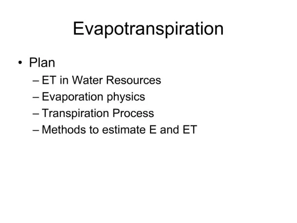
2. Why we need evapotranspiration(ET)? ET =“How wet is there?” Water resources management & drought monitoring - Water resource crisis is biggest problem in 21st century. ---- ET consumes precious water resources!!! - Fire risk assessment Improve Models - ET serves as input data or validation data for climate model. - Validation of ecosystem model (Biome-BGC, RHESSys, etc.) Diagnose environment - Urbanization  change energy budget  hot city? (like Tokyo in summer) - Cut/plant forest  change energy budget  change climate & productivity - Global warming  ET increase? Decrease?

3. Why ET by satellite? • Score table of three approaches to ET • -------------------------------------------------------------------------------------------------------- Observation model satellite RS-------------------------------------------------------------------------------------------------------- • Time coverage Good!Good!Poor… • Spatial coverage Poor… So-so. Good! • Accuracy Good! So-so. So-so. • Cost efficiency Poor… So-so. So-so. • -------------------------------------------------------------------------------------------------------- • Particular advantage of satellite RS: • Not influenced by water re-distribution (e.g., irrigation)- Strong at phenology

4. Why is Aqua/MODIS good? • Frequent global coverage (every day + combination with Terra/MODIS) • Afternoon overpass … dry condition becomes clearer than morning • High-spatial resolution (1km)cf. Microwave remote sensing • High-precision of temperature and vegetation indices cf. NOAA/AVHRR • albedo and emissivity are available. cf.NOAA/AVHRR • Atmospheric information is available from other sensors on Aqua • AIRS/AMSU/HSB…… accurate atmospheric profile!!!

5. Outline of the Project Final ProductEF (Evaporation Fraction) values- 8 day-period, 1km resolution, globally - by Aqua (EOS-PM)/MODIS Requirements for the algorithm - Stand alone: It can operate only with optical satellite sensor data - Flexible: It can ingest any other reliable data, if available. - Simple: It is simply constructed to reduce computational load. - Scalable: It can give daily information of ET from instants data. - Versatility: It can operate regardless of climate and biome. - Sensor Independence: It can co-operate with other sensors with same logic.

6. What is Evaporation Fraction? Available Energy Ground heat transfer Net radiation (radiation absorbed on the land) • Fractional value is representative for “wetness”. • Scalability of instantaneous observation to longer period. • Accurate estimate of Q is difficult. Potential for coupling with Terra-MODIS (AM overpass) From: Crago, 1996, “Scaling up in Hydrology using Remote Sensing”

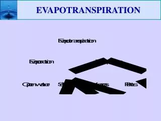
7. MODIS-ET Model Landscape Actual landscape: mixture of forest, farm, grassland, road, etc. Simplification ETbare ETveg ET = fveg ETveg + (1 –fveg) ET soil Qveg Qbare EF = fveg EFveg + (1 –fveg)  EFbare QQ Fraction of bare soil: 1.0 - fveg Fraction of vegetation: fveg

8. How do we get it? - Temperature on vegetation: Tveg (S) - Incoming solar radiation: PAR (T) - radiative transfer of atmosphere(T) • VI-Ts diagram (S) Qveg Qbare EF = fveg EFveg + (1 –fveg)  EFbare QQ We want this! - Vegetation Index …NDVI or EVI (S) Note: (S) …. Derived from Satellite (T) …. Estimated theoretically

9. EstimatingEFveg(1) Concept Central concept: Evaporation from vegetation (transpiration) is mostly controlled by stomata opening (canopy resistance). Assuming complementary relationship (ET + PETPM = 2PETPT; PETPM=Penman’s PET; PETPT=Priestley-Taylor’s PET), we can get: Constant. 1.26 Derivative of saturated vapor pressure curve (change with T) αΔ EFveg =  Δ + γ ( 1 + rc / 2 ra) Aerodynamic resistance Psychrometric constant (slightly change with T) Canopy resistance

10. EstimatingEFveg(2) Canopy Resistance Model 1 / rc = f1(T) f2(VPD) f3(PAR) f4()/ rcMIN Ideally, Temperature Solar radiation Humidity Soil water Actually, Change of VI 1 / rc = f1(T) f3(PAR) / rcMIN

11. EstimatingEFbare satellite image Ts Tbare max Warm Edge Wind speed Tbare Window Tbare max – Tbare EFbare=  Tbare max – Tbare min Tveg=Tbare min Air temperature VI VImin VImax VI VI-Ts diagram (Nemani & Running, 1989; 1993) Qbare0– ET Tbare =  + Ta 4εσTa3 (1- CG) +  Cp/ra bare

12. Data Stream Satellite data VI albedo Channel reflectance Thermal IR Ts Tbare max Tbare Ta VI Ts VI-Ts diagram EFbare VI fveg OrbitTa Rd PAR Radiative transfer model RdTaalbedo Qbare Qbare0 Qveg Radiation budget EF Qbare Tbare max Ta U50m ra Energy budget Ta PAR Conductance model rc Ta ra rc Penman-Monteith & Complementary relation EFveg

13. Prototype • NOAA/AVHRR 14-day composite (1km resolution) • Window size: 21km*21km • Validation 13 sites of AmeriFlux

15. Validation Comparison of estimated EF by AVHRR and observed EF at AmeriFlux sites  site (symbol) type data size R 2 bias standard error  Harvard Forest DBF 28 0.75 -0.05 0.13 Walker Branch DBF 29 0.88 0.01 0.13 Willow Creek DBF 8 0.80 -0.14 0.18 WLEF Tower DBF 17 0.89 -0.18 0.20 Blodgett ENF 11 0.30 -0.12 0.21 Duke Forest ENF 13 0.70 0.04 0.19 Howland ENF 20 0.84 -0.02 0.10 Metolius ENF 15 0.20 -0.12 0.23 Bondville Crop 37 0.81 -0.07 0.19 Ponca Crop 6 0.36 -0.10 0.31 Little Washita Grass 20 0.86 0.04 0.14 Shidler Grass 10 0.91 -0.03 0.12 Ski Oaks Shrub 16 0.29 -0.07 0.17 all sites --- 230 0.74 -0.05 0.17

16. Only NDVI Full algorithm Validation for each landcover type Test of simplified algorithm

17. Prototype with Terra/MODIS Day233, 2000North USA (Tile H10-12V04)