Download
1 / 46
480 likes | 702 Vues
Purchasing Power Parity – Chapter 12 BOP Adjustments – Chapter 13 Exchange Rate Systems – Chapter 15. Purchasing Power Parity. The simplest concept of PPP is the law of one price Law of one price

E N D
Purchasing Power Parity – Chapter 12 BOP Adjustments – Chapter 13 Exchange Rate Systems – Chapter 15
Purchasing Power Parity • The simplest concept of PPP is the law of one price • Law of one price • An identical good should cost the same in all nations, assuming costless shipping and no barriers. • Before the costs of a good in different nations can be compared, its price must be converted into a common currency. • Once converted, the price of an identical good from any 2 countries must be identical
Theoretically, the pursuit of profits tends to equalize the price of an identical product in different nations. • Example: • Assume machine bought in Switzerland are cheaper than the same machine bought in US after converting francs to dollars. • Swiss exporters can gain by purchasing machine in Switzerland at low price & sell them in US at high price • This transactions would P in Switzerland and P in US until the price of machine be equal in the 2 countries – law of price prevail. • Single price might not apply in practice
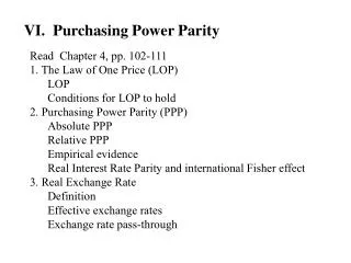
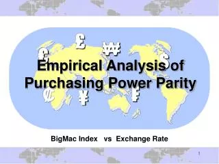
Big Mac Index & Law of One Price • An attempt to measure the true equilibrium value of a currency based upon one product – Big Mac hamburger. • According to law of one price – a Big Mac should cost the same in a given currency wherever it is purchased, suggesting that the prevailing market exchange-rate is the true equilibrium rate.
Big Mac Index suggests that the market-exchange rate between $ and Yen is in equilibrium when it equates the prices of hamburger in US and Jpn. • Implying that Big Macs would cost the same in each country when prices are converted to $. • If the cost is not same – law of one price does not hold. • In this case, Yen is said to be over – or – undervalued compared to $. • Thus Big Mac Index could be used to determine the extent which the market exchange rate differs from the true equilibrium exchange rate.
The dollar price of BM different than the US level in all countries surveyed – violating the law of one price.. • BM cost $3.06 in US. In Norway the dollar equivalent price of BM = $6.06 (overvalued 98%). In China BM = $1.27 (undervalued 59%). • There are many flaws in this index butserves as an approximation of the currency strength
Purchasing Power Parity • The PPP theory provides a generalized explanation of exchange rates based on the prices of many goods. • Simply the application of the law of one price to national price levels. It says that: • Exchange rates are related to differences in the level of prices between two countries • Thus the changes in relative national price levels determine changes in exchange rates over the long run • Predicts that foreign-exchange value of a currency tends to appreciate or depreciate at a rate equal to the difference between foreign & domestic inflation.
The PPP in symbols: • P = price indexes of the US and Switzerland • 0 = base period and 1 = period 1 • So = equilibrium exchange rate existing in the base period • S1 = estimated target as which the actual rate should be in the future
Example: Price indexes of the US & Switzerland and equilibrium exchange rate is as follows: Pus0 = 100 Pus1 = 200 Ps0 = 100 Ps1 = 100 So = $0.50 New equilibrium exchange rate for period 1 = S1 = $0.50 (200/100) = $0.50 (2) = $1.00 (100/100) US inflation rate rose 100%, whereas Switzerland remain unchanged. PPP requires that $ depreciate against franc by an amount to the difference in the percentage rates of inflation in US and Switzerland. The dollar must depreciate by 100 % from $0.50 per franc to $1 per franc.
Purchasing Power Parity • Although the PPP theory can be helpful in forecasting appropriate levels to which currency values should be adjusted, there are some limitations. • Limitations of the theory • Overlooks the fact that exchange-rate movements may be influenced by investment flows • Choosing the appropriate price index (consumer or producer price index) • Determining the equilibrium period to use as a base • Government policy interference
13 Balance-of-Payments Adjustments
The adjustment mechanism works for the return to equilibrium after the initial equilibrium has been disrupted. • Payments adjustment takes 2 different forms: • there are adjustment factors that automatically promote equilibrium. • if automatic adjustment unable to restore equilibrium, discretionary government policies may be adopted. There are 3 main adjustment variables for automatic adjustment of BOP : prices, interest rates & income.
Price Adjustments • Original theory of balance-of-payments adjustment: David Hume (1711–1776) • A nation’s balance of payments tends to move toward equilibrium automatically • Role that adjustments in national price levels play in promoting balance-of-payments equilibrium
Gold Standard • Existed from the late 1800s to the early 1900s • Characterized by three conditions • Each member nation’s money supply consisted of gold or paper money backed by gold • Each member nation defined the official price of gold in terms of its national currency and was prepared to buy and sell gold at that price • Free import and export of gold was permitted • Under these conditions, a nation’s money supply was directly tied to its BOP.
Deficit nation • Gold outflow; reduction in money supply and thus its price level, till balance-of-payments equilibrium is restored • Surplus nation • Gold inflows and an increase in its money supply till equilibrium is restored
BOP Price Adjustment • Under the classical gold standard, the BOP is linked to a nation’s money supply, which is linked to its domestic price level. • If BOP deficit: - experience gold outflow which would reduce money supply & price level. - Nation’s international competitiveness improved so that its exports ↑ & imports ↓. - the process continues until P level had risen to the point where BOP equilibrium was restored.
BOP Price Adjustment • If BOP surplus: - experience gold inflow which would ↑money supply & price level. - the process continues until P level had risen to the point where BOP equilibrium was restored. The linkages BOP-MS-P level- shows that over time BOP equilibrium tends to be achieved automatically
Income Adjustments • Criticism of classical theory – it almost completely neglected the effect of income adjustments. • Theory of income determination – John Maynard Keynes (1930s) provide the explanation. • Under fixed exchange rates • Influence of income changes in surplus and deficit nations would help restore payments equilibrium automatically. • Persistent payments imbalance – a surplus nation will experience rising income and will ↑ imports. • A deficit nation will experience fall in income & reduced imports • The effects of income changes on imports levels will reverse the disequilibrium in the BOP.
Foreign repercussion effect • Income-adjustment mechanism further modified to include the impact that changes in domestic expenditures and income levels have on foreign economies. • Significant for major trading nations • E.g. US & Canada initially at BOP equilibrium • Suppose US ↑ imports from Canada ↑ Canada’s exports ↓US income (↓imports means that ↓Canada’s exports ) & ↑ Canada income (↑ imports means that ↑ in US exports) • Process repeated again and again until the BOP achieve equilibrium • Foreign repercussion effect depends on the economic size of a country and the extent of international trade.
Income Determination in an Open Economy • The condition for equilibrium income is represented by: S + M (leakages) = I + X (injections) Rearrange the terms S – I = X – M Assume M are dependent on domestic income ∆M = m∆Y where m= marginal propensity to import
To derive foreign-trade multiplier Let the injections & leakages rise by the same amount which is represented by; ∆S + ∆M = ∆I + ∆X Given ∆S= s ∆Y and ∆M = m ∆Y (s + m) ∆Y = ∆I + ∆X Holding exports constant (∆X=0), the induced change in income is equal to ∆Y = 1 X ∆I (s + m)
Implications of the foreign trade multiplier • Have 2 curves: (S – I) = positively sloped because ∆S are directly related to ∆Y, investment being unaffected. (X – M) = negatively sloped because it is assumed that ∆M are directly related to ∆Y, exports remaining constant. When M are subtracted from X, so (X-M) curve is downward sloping. • The equilibrium condition of an open economy with no government with fixed exchange rates system is (X-M) = (S-I)
Domestic income & trade balance effects of an increase in exports & investment S-I, X-M (dollars) 400 300 F 200 S - I S – I ’ G 100 E Income 0 200 400 600 800 1,000 1,200 1,800 2,000 1,400 1,600 I -100 X’ - M -200 H X - M -300 -400
a) Increase in Exports • Equilibrium income = $1,000 • Suppose X ↑ by $200 (X – M ) shifts upward by $200 to (X’-M). • Y ↑ generating increases in M and S. • Domestic equilibrium established at Y=$1,400 where (S-I)=(X’-M). • The trade account no longer balance because there is trade surplus = $100 ( < than $200 rise in X because part of the surplus is offset by increases in M induced by rise in Y from $1,000 to $1,400.
b) Increase in Investment • Equilibrium income = $1,000 • Suppose I ↑ by $200 (S – I ) shifts downward to (S- I’). • Domestic equilibrium established at Y=$1,400 where (S-I’)=(X-M). • Stimulates rise in M thus producing trade deficit of $100. • An autonomous ↑ in domestic I (or government expenditures) increases domestic Y but at the expense of a BOP deficit. • Thus under system of fixed exchange rates, the impact of domestic policies on BOP cannot be overlooked.
15 Exchange-Rate Systems
This chapter surveys the exchange rates practices that are currently being used. • In choosing exchange rate system, a nation must decide whether: • to allow its currency to be determined by market forces (floating rate –independently, group of currencies or crawl) or • to be fixed (pegged) against some standard of value.
Types of Exchange Rate Systems • Fixed exchange rate system • Adjustable peg • Floating exchange rate system • Managed floating rates • The crawling peg
Fixed Exchange-Rate System • General practice until the 1970s • Changes in national exchange rates initiated by domestic monetary authorities when long-term market forces warranted it. • Primarily used by small, developing nations • Currencies are anchored to a key currency such ass US dollar (traded in world money markets, relatively stable & widely accepted as means of international settlements) • Benefits of anchoring to key currencies • Developing nations can stabilize the domestic-currency prices of their imports and exports • Exerts restraint on domestic policies and reduces inflation
The government assigned their currencies a par value. • The exchange rate is only allowed to fluctuate within the very limited band compared to the par value (1%). • Government will monitor the exchange rate by interfering in the forces DD and SS in foreign exchange market. • It is very rigid exchange rate system but could to some extent reduce frequent fluctuation in the exchange rate. • Weakness – involve very expensive maintenance cost because involves buying back of currencies when there is depreciation.
In maintaining FER, a nation can : • Anchor to a single currency • Developing nations with a single industrial-country partner • Anchoring to a group or basket of currencies • Developing nations with more than one major trading partner • Helps to average out fluctuations • Anchoring to the special drawing right (SDR) • Basket of four currencies • Increased stability
Under FER system, a nation’s monetary authority may decide to pursue BOP equilibrium by devaluing or revaluing its currency. • Devaluation • The purpose of devaluation is to cause home currency’s exchange value to depreciates, thus counteracting a payments deficit • Revaluation • Home currency’s exchange value to appreciates, thus counteracting a payments surplus • Decisions to be made before implementation • Necessity of the step • Timing of adjustment • Magnitude of adjustment
Advantages of FER system: • Simplicity & clarity of exchange-rate target • Automatic rule for the conduct of monetary policy • Disadvantages of FER system: • Loss of independent of monetary system • Vulnerable to speculative attacks
Bretton Woods System of Fixed Exchange Rates • Adjustable pegged exchange rates lasted from 1946 to1973. • A kind of semifixed exchange rate system (neither completely FER nor floating rates). • Main features: -Currencies tied to each other - When there is BOP disequilibrium: could repeg exchange rate via revaluation or devaluation. - Operational difficulties: • Conflicting objectives, Magnitude of adjustments, Difficulties in estimating equilibrium rates and Speculation
Floating Exchange Rates • Currency prices are established daily in the foreign-exchange market • Without restrictions imposed by government policies • There is equilibrium exchange rate that equates the demand for and supply of the home currency • Unlike FER, floating rates are not characterized by par values & official exchange rates
Arguments For and Against Floating Rates • Advantages • Simplicity • Continuous adjustment in the balance of payments • Adverse effects of prolonged disequilibriums are minimized • Partially insulates the home economy from external forces • Freedom to pursue policies that promote domestic balance • Disadvantages • Unregulated market leads to wide fluctuations in currency values • Prohibitively high cost of hedging • Flexibility to set independent policies leading to inflationary bias
Managed Floating Rates • Adopted by US & other industrial nations in 1973 following the breakdown of the fixed exchange rates system • Informal guidelines established by IMF (1973) • Under managed floating, a nation: • Can alter the degree of intervention • Can intervene to reduce short-term fluctuations: Leaning against the wind • Should not act aggressively with respect to their currency exchange rates • Can choose target rates and intervene to support them
Under a managed float • Market intervention is used to stabilize exchange rates in the short run • In the long run, a managed float allows market forces to determine exchange rates • Example: Theory of a managed float in a two-country framework
A. Long-term change Suppose US income DD for Swiss products increase DD for francs to D1 excess DD results in a rise in exchange rate to $0.60 per franc (Qd=Qs). LR movements of exchange rate are determined by the supply & demand for various currencies B. Short-term fluctuation Suppose US investors DD additional francs which gives high interest rates DD shift to D1 Suppose Swiss interest rates fall DD for francs revert to Do. Under floating rates – the dollar price of francs will rise from $0.50 to $0.60 per franc & then fall back to $0.50 per franc. Under managed floating rates Central bank will intervene in response to temporary disturbance to keep the exchange rate at the LR equilibrium ($0.50 per franc). When DD= DI, CB will sell francs to meet excess DD. When DD reverts back to Do – no intervention required. Managed floating exchange rates
The Crawling Peg • Means that a nation makes small, frequent changes in the par value of its currency to: • Correct BOP disequilibriums • Deficit & surplus nations keep on adjusting until the desired exchange rate level is attained. • Used primarily by nations having high inflationrates (believe that pegging system can operate in an inflationary environment only if there is provision for frequent changes in the par values)
The Crawling Peg • Supporters of crawling peg argue that the system combines • The flexibility of floating rates with the stability of fixed rates • More responsive to changing competitive conditions • Avoids changes that are frequently wide of the mark • Frustrates speculators with their irregularity • IMF view • Hard to apply this system to industrialized nations whose currencies serve as a source of international liquidity
Summary • Purchasing Power Parity • BOP Adjustments – Price and Income • Exchange Rate Systems - Fixed exchange rate system - Adjustable peg - Floating exchange rate system - Managed floating rates - Crawling peg