Download
1 / 45
470 likes | 959 Vues
The Short-Run Macro Model. Spending is very important in short-run The more income households have, the more they will spend Spending depends on income But the more households spend, the more output firms will produce More income they will pay to their workers

E N D
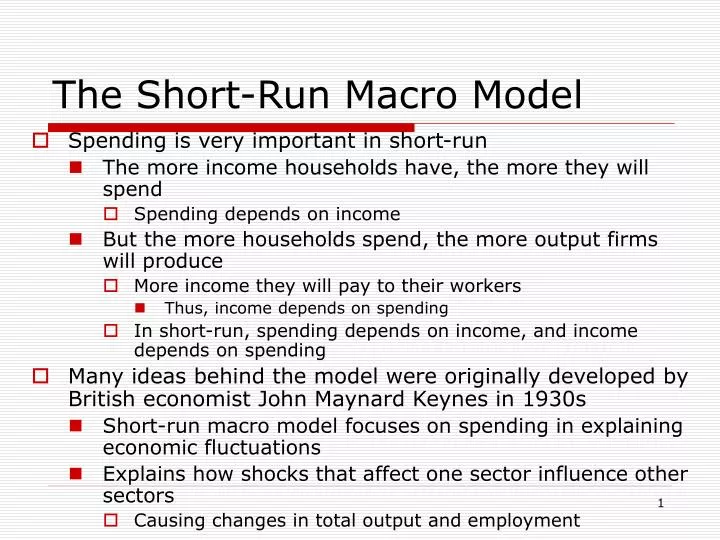
The Short-Run Macro Model • Spending is very important in short-run • The more income households have, the more they will spend • Spending depends on income • But the more households spend, the more output firms will produce • More income they will pay to their workers • Thus, income depends on spending • In short-run, spending depends on income, and income depends on spending • Many ideas behind the model were originally developed by British economist John Maynard Keynes in 1930s • Short-run macro model focuses on spending in explaining economic fluctuations • Explains how shocks that affect one sector influence other sectors • Causing changes in total output and employment
Thinking About Spending • Spending on what? • In short-run macro model, focus on spending in markets for currently produced U.S. goods and services • Things that are included in U.S. GDP • Need to organize our thinking about markets that contribute to GDP • What’s the best way to categorize all these buyers into larger groups so we can analyze their behavior? • Macroeconomists have found that the most useful approach is to divide those who purchase the GDP into four broad categories • Households, whose spending is called consumption spending (C) • Business firms, whose spending is called planned investment spending (IP) • Government agencies, whose spending on goods and services is called government purchases (G) • Foreigners, whose spending we measure as net exports (NX) • Should we look at nominal or real spending? • When discuss “consumption spending,” we mean “real consumption spending”
Consumption Spending • Natural place for us to begin our look at spending is with its largest component • Consumption spending • Total consumption spending is sum of spending by over a hundred million U.S. households • What determines total amount of consumption spending? • One way to answer is to start by thinking about yourself or your family • What determines your spending in any given month, quarter, or year?
Disposable Income • First thing that comes to mind is your income • The more you earn, the more you spend • It’s not exactly your income per period that determines your spending • But rather what you get to keep from that income after deducting any taxes you have to pay • If we start with income you earn, deduct all tax payments, and then add in any transfer received, would get your disposable income • Income you are free to spend or save as you wish • Disposable Income = Income – Tax Payments + Transfers Received • Can be rewritten as • Disposable Income = Income – (Taxes – Transfers) or • Disposable Income = Income – Net Taxes • For almost any household, a rise in disposable income—with no other change—causes a rise in consumption spending
Wealth • Given your disposable income, how much of it will you spend and how much will you save? • Will depend, in part, on your wealth • Total value of your assets minus your outstanding liabilities • In general, a rise in wealth—with no other change—causes a rise in consumption spending
The Interest Rate • Interest rate is reward people get for saving, or what they have to pay when they borrow • All else equal, a rise in interest rate causes a decrease in consumption spending • Relationship between interest rate and consumption spending applies even for people who aren’t “savers” in the common sense of term • Whether you are earning interest on funds you’ve saved, or paying interest on funds you’ve borrowed • The higher the interest rate, the lower is consumption spending • In macroeconomics, household saving is the part of disposable income that a household doesn’t spend • Whether it’s put in bank or used to pay off a loan
Expectations • Expectations about future would affect your spending as well • All else equal, optimism about future income causes an increase in consumption spending • Other variables influence your consumption spending • Including inheritances you expect to receive over your lifetime, and even how long you expect to live • Disposable income, wealth, and interest rate are the three key variables • In macroeconomics, we use phrases like “disposable income,” “wealth,” or “consumption spending” to mean the total disposable income, total wealth, and total consumption spending of all households in the economy combined • All else equal, consumption spending increases when • Disposable income rises • Wealth rises • Interest rate falls
7,000 2000 6,000 1995 Real Consumption Spending ($ Billions) 5,000 1990 1985 4,000 3,000 3,000 4,000 5,000 6,000 7,000 Real Disposable Income ($ Billions) Figure 1: U.S. Consumption and Disposable Income, 1985-2004
Consumption and Disposable Income • Of all the factors that influence consumption spending, most important and stable determinant is disposable income • Relationship between consumption and disposable income is almost perfectly linear—points lie remarkably close to a straight line • This almost-linear relationship between consumption and disposable income has been observed in a wide variety of historical periods and a wide variety of nations • Vertical intercept in Figure 2 is called • Autonomous consumption spending • Part of consumption spending that is independent of income
The consumption function shows the (linear) relationship between real consumption spending and real disposable income 8,000 7,000 6,000 The vertical intercept ($2,000 billion) is autonomous consumption spending . . . 5,000 Real Consumption Spending ($ Billions) 4,000 3,000 and the slope of the line (0.6) is the marginal propensity to consume. 2,000 1,000 1,000 2,000 3,000 4,000 5,000 6,000 7,000 8,000 Real Disposable Income ($ Billions) Figure 2: The Consumption Function Consumption Function 600 1,000
Consumption and Disposable Income • Second important feature of Figure 2 is the slope • Shows change along vertical axis divided by change along horizontal axis as we go from one point to another on the line • Slope = Δ Consumption ÷ Disposable Income • Economists have given this slope a special name • Marginal propensity to consume, or MPC • Can think of MPC in three different ways, but each of them has the same meaning • Slope of consumption function • Change in consumption divided by change in disposable income • Amount by which consumption spending rises when disposable income rises by one dollar • Logic suggests that the MPC should be larger than zero, but less than 1 • We will always assume that 0 < MPC < 1
Representing Consumption with an Equation • Sometimes, we’ll want to use an equation to represent straight-line consumption function • C = a + b x (Disposable Income) • Where C is consumption spending • Term a is vertical intercept of consumption function • Represents theoretical level of consumption spending at disposable income=0, or autonomous consumption spending • Term b is slope of consumption function • Marginal propensity to consume (MPC)
Consumption and Income • Consumption function is an important building block • Consumption is largest component of spending, and disposable income is most important determinant of consumption • If government collected no taxes, total income and disposable income would be equal • So that relationship between consumption and income on the one hand, and consumption and disposable income on the other hand, would be identical • Consumption-income line • Line showing aggregate consumption spending at each level of income or GDP • When government collects a fixed amount of taxes from household • Line representing relationship between consumption and income is shifted downward by amount of tax times marginal propensity to consume (MPC) • Slope of this line is unaffected by taxes and is equal to MPC
Real Consumption Spending ($ Billions) 5,600 2. The line has the same slope as the consumption function in Figure 2. . . 5,000 4,000 3,000 2,000 1. To draw the consumption-income line, we measure real income (instead of real disposable income) on the horizontal axis. 3. but a different vertical intercept. 1,000 2,000 4,000 6,000 8,000 Real Income ($ Billions) Figure 3: The Consumption-Income Line Consumption-Income Line B A 600 1,000
Shifts in the Consumption-Income Line • If income increases and net taxes remain unchanged, disposable income will rise, and consumption spending will rise along with it • But consumption spending can also change for reasons other than a change in income, causing consumption-income line itself to shift • Mechanism works like this
Shifts in the Consumption-Income Line • Can summarize our discussion of changes in consumption spending as follows • When a change in income causes consumption spending to change, we move along consumption-income line • When a change in anything else besides income causes consumption spending to change, the line will shift • All changes that shift the line—other than a change in taxes—work by increasing or decreasing autonomous consumption (a)
8,000 Real Consumption Spending ($ Billions) Consumption-Income Line When Net Taxes = 500 7,000 6,000 5,000 4,000 3,000 Consumption-Income Line When Net Taxes = 2,000 2,000 1,000 2,000 4,000 6,000 8,000 Real Income ($ Billions) Figure 4: A Shift in the Consumption-Income Line
Table 3: Changes in ConsumptionSpending and the Consumption–Income Line
Investment Spending • In definition of GDP, word investment by itself (represented by the letter “I” by itself) consists of three components • Business spending on plant and equipment • Purchases of new homes • Accumulation of unsold inventories • In short-run macro model, we define (planned) investment spending (IP) as • Plant and equipment purchases by business firms, and new home construction • Inventory investment is treated as unintentional and undesired • Excluded from definition of investment spending • For now, we regard investment spending (IP) as a given value, determined by forces outside of our model
Government Purchases • Include all goods and services that government agencies—federal, state, and local—buy during year • In short-run macro model, government purchases are treated as a given value • Determined by forces outside of model
Net Exports • If we want to measure total spending on U.S. output, we must also consider international sector • U.S. exports • But international trade in goods and services also requires us to make an adjustment to other components of spending • In sum, to incorporate international sector into our measure of total spending, we must add U.S. exports, and subtract U.S. imports • Net Exports = Total Exports – Total Imports
Net Exports • By including net exports, simultaneously ensure that we have • Included U.S. output that is sold to foreigners, and • Excluded consumption, investment, and government spending on output produced abroad • For now, we regard net exports as a given value, determined by forces outside of our analysis • Important to remember that net exports can be negative • United States has had negative net exports since 1982 • Imports are greater than exports
Summing Up: Aggregate Expenditure • Aggregate expenditure • Sum of spending by households, businesses, government, and foreign sector on final goods and services produced in United States • Aggregate expenditure = C + IP + G + NX • C stands for household consumption spending, IP for investment spending, G for government purchase, and NX for net exports • Plays a key role in explaining economic fluctuations • Why? • Because over several quarters or even a few years, business firms tend to respond to changes in aggregate expenditure by changing their level of output
Income and Aggregate Expenditure • Relationship between income and spending is circular • Spending depends on income, and income depends on spending • We take up the first part of that circle • How total spending depends on income • Notice that aggregate expenditure increases as income rises • But notice also that rise in aggregate expenditure is smaller than rise in income • When income increases, aggregate expenditure (AE) will rise by MPC times change in income • ΔAE = MPC x Δ GDP • We’ve used ΔGDP to indicate change in total income • Because GDP and total income are always the same number
Finding Equilibrium GDP • Method of finding equilibrium in short-run is very different from anything you’ve seen before • Starting point in finding economy’s short-run equilibrium is to ask ourselves what would happen, hypothetically, if economy were operating at different levels of output • When aggregate expenditure is less than GDP, output will decline in future • Any level of output at which aggregate expenditure is less than GDP cannot be equilibrium GDP • When aggregate expenditure is greater than GDP, output will rise in future • Any level of output at which aggregate expenditure exceeds GDP cannot be equilibrium GDP • In short-run, equilibrium GDP is level of output at which output and aggregate expenditure are equal
Inventories and Equilibrium GDP • When firms produce more goods than they sell, what happens to unsold output? • Added to their inventory stocks • Change in inventories during any period will always equal output minus aggregate expenditure • Find output level at which change in inventories is equal to zero • AE < GDP ΔInventories > 0 GDP↓ in future periods • AE > GDP ΔInventories < 0 GDP↑ in future periods • AE = GDP ΔInventories = 0 No change in GDP • Equilibrium output level is one at which change in inventories equals zero
Finding Equilibrium GDP With A Graph • Figure 5 gives an even clearer picture of how equilibrium GDP is determined • Lowest line, C, is consumption-income line • Next line, labeled C + IP, shows sum of consumption and investment spending at each income level • Next line adds government purchases to consumption and investment spending, giving us C + IP + G • Top line adds net exports, giving us C + IP + G + NX, or aggregate expenditure
8,000 Real Aggregate Expenditure ($ Billions) 7,000 5. to get the aggregate expenditure line. 6,000 4. and net exports (NX) . . . 5,000 3. government purchases (G) . . . 4,000 3,000 2,000 2. then add planned investment (IP) . . . 1,000 1. Start with the consumption-income line, 2,000 4,000 6,000 8,000 Real GDP ($ Billions) Figure 5: Deriving the Aggregate Expenditure Line C + IP + G + NX C + IP + G C + IP C
Finding Equilibrium GDP With A Graph • Figure 6 shows a graph in which horizontal and vertical axes are both measured in same units, such as dollars • Also shows a line drawn at a 45° angle that begins at origin • 45° line is a translator line • Allows us to measure any horizontal distance as a vertical distance instead • Now we can apply this geometric trick to help us find the equilibrium GDP
1. Using a 45-degree line . . . 3. into an equal vertical distance (BA). 2. we can translate any horizontal distance (such as 0B) . . . Fig. 6 Using a 45° Line to Translate Distances A 45° 0 B
Finding Equilibrium GDP With A Graph • Figure 7 shows how we can apply geometric trick to help us find equilibrium GDP • At any output level at which aggregate expenditure line lies below 45° line, aggregate expenditure is less than GDP • If firms produce any of these out put levels, inventories will grow, and they will reduce output in the future • At any output level at which aggregate expenditure line lies above 45° line, aggregate expenditure exceeds GDP • If firms produce any of these output levels, inventories will decline, and they will increase their output in the future • We have thus found our equilibrium on graph • Equilibrium GDP is output level at which aggregate expenditure line intersects 45° line • If firms produce this output level, their inventories will not change, and they will be content to continue producing same level of output in the future
Real Aggregate Expenditure ($ Billions) Increase in Inventories 9,000 8,000 7,000 6,000 Decrease in Inventories 5,000 4,000 3,000 2,000 1,000 Real GDP ($ Billions) 2,000 4,000 6,000 8,000 Figure 7: Determining Equilibrium Real GDP A C + IP + G + NX H E K Total Output Aggregate Expenditure J Aggregate Expenditure Total Output 45°
Equilibrium GDP and Employment • When economy operates at equilibrium, will it also be operating at full employment? • Not necessarily • It would be quite a coincidence if our equilibrium GDP happened to be output level at which entire labor force were employed • In short-run macro model, cyclical unemployment is caused by insufficient spending • As long as spending remains low, production will remain low, and unemployment will remain high • In short-run macro model, economy can overheat because spending is too high • As long as spending remains high, production will exceed potential output, and unemployment will be unusually low • Aggregate expenditure line may be low, meaning that in short-run, equilibrium GDP is below full employment • Or aggregate expenditure may be high, meaning that in short-run, equilibrium GDP is above full-employment level
When the aggregate expenditure line is low . . . Aggregate Expenditure ($ Billions) Real GDP ($ Billions) equilibrium output ($6,000) is less than potential output, Real GDP ($ Billions) Number of Workers and equilibrium employment is less than full employment. Figure 8: Equilibrium GDP Can Be Less Than Full Employment GDP Aggregate Production Function AELOW B F $7,000 $7,000 E cyclical unemployment = 25 million $6,000 A 45° $7,000 100 Million $6,000 75 Million Potential GDP Full Employment
Aggregate Expenditure ($ Billions) Real GDP ($ Billions) When the aggregate expenditure line is high . . . and equilibrium employ- ment is greater than full employment. equilibrium output ($8,000) is greater than potential output, Real GDP ($ Billions) Number of Workers Figure 9: Equilibrium GDP Can Be Greater Than Full-Employment GDP AEHIGH Aggregate Production Function E' H $8,000 B $7,000 $7,000 F $7,000 $7,000 100 Million $8,000 135 Million Potential GDP Full Employment
A Change in Investment Spending • Suppose equilibrium GDP in an economy is $6,000 billion, and then business firms increase their investment spending on plant and equipment by $1,000 billion • What will happen? • Sales revenue at firms that manufacture investment goods will increase by $1,000 billion • Each time a dollar in output is produced, a dollar of income (factor payment) is created • What will households do with their $1,000 billion in additional income? • What they will do depends crucially on marginal propensity to consume (MPC) • Assume MPC = 0.6
A Change in Investment Spending • When households spend an additional $600 billion, firms that produce consumption goods and services will receive an additional $600 billion in sales revenue • Which will become income for households that supply resources to these firms • With an MPC of 0.6, consumption spending will rise by 0.6 x $600 billion = $360 billion, creating still more sales revenue for firms, and so on and so on… • Increase in investment spending will set off a chain reaction • Leading to successive rounds of increased spending and income • At end of process, when economy has reached its new equilibrium • Total spending and total output are considerably higher
Increasein Annual GDP Figure 10: The Effect of a Change in Investment Spending 2,500 2,306 2,176 1,960 1,600 1,000 Initial Rise in IP After Round 2 After Round 3 After Round 4 After Round 5 After All Rounds
The Expenditure Multiplier • Whatever the rise in investment spending, equilibrium GDP would increase by a factor of 2.5, so we can write • ΔGDP = 2.5 x ΔIP • Expenditure multiplier is number by which the change in investment spending must be multiplied to get change in equilibrium GDP • Value of expenditure multiplier depends on value of MPC • Simple formula we can use to determine multiplier for any value of MPC • 1 / (1 – MPC) • Using general formula for expenditure multiplier, can restate what happens when investment spending increases
The Expenditure Multiplier • A sustained increase in investment spending will cause a sustained increase in GDP • Multiplier process works in both directions • Just as increases in investment spending cause equilibrium GDP to rise by a multiple of the change in spending • Decreases in investment spending cause equilibrium GDP to fall by a multiple of the change in spending
Other Spending Shocks • Shocks to economy can come from other sources besides investment spending • Suppose government agencies increased their purchases above previous levels • Besides planned investment and government purchases, there are two other components of spending that can set off the same process • An increase in net exports (NX) • A change in autonomous consumption • Changes in planned investment, government purchases, net exports, or autonomous consumption lead to a multiplier effect on GDP • Expenditure multiplier is what we multiply initial change in spending by in order to get change in equilibrium GDP
Other Spending Shocks • Following four equations summarize how we use expenditure multiplier to determine effects of different spending shocks in short-run macro model
A Graphical View of the Multiplier • Figure 11 illustrates multiplier using aggregate expenditure diagram • An increase in autonomous consumption spending, investment spending, government purchases, or net exports will shift aggregate expenditure line upward by increase in spending • Causing equilibrium GDP to rise • Increase in GDP will equal initial increase in spending times expenditure multiplier
Real Aggregate Expenditure ($ Billions) 9,000 8,000 7,000 6,000 5,000 4,000 3,000 2,000 1,000 Real GDP ($ Billions) 2,000 4,000 6,000 8,000 Figure 11: A Graphical View of the Multiplier AE2 F AE1 E $1,000 Increase in Equilibrium GDP $2,500 Billion 45°
The Effect of Fiscal Policy • In classical model fiscal policy—changes in government spending or taxes designed to change equilibrium GDP—is completely ineffective • In short-run, an increase in government purchases causes a multiplied increase in equilibrium GDP • Therefore, in short-run, fiscal policy can actually change equilibrium GDP • Observation suggests that fiscal policy could, in principle, play a role in altering path of economy • Indeed, in 1960s and early 1970s, this was the thinking of many economists • But very few economists believe this today