Download

1 / 23
230 likes | 328 Vues
Twenty Years of Eddies in the Alaska Coastal Current. Albert J. Hermann Joint Institute for the Study of the Atmosphere and the Oceans, UW/NOAA/PMEL, 7600 Sand Point Way NE, Seattle, WA 98115) Phyllis J. Stabeno (PMEL) Michael Spillane (JISAO/NOAA/PMEL). The Problem.

E N D
Twenty Years of Eddies in the Alaska Coastal Current Albert J. Hermann Joint Institute for the Study of the Atmosphere and the Oceans, UW/NOAA/PMEL, 7600 Sand Point Way NE, Seattle, WA 98115) Phyllis J. Stabeno (PMEL) Michael Spillane (JISAO/NOAA/PMEL)
The Problem • Large interannual variability observed in the structure of the Alaska Coastal Current (ACC) and associated fish stocks • Eddy statistics in the ACC (number, size, strength) affect larval paths and may affect subsequent recruitment • Can Lagrangian/Eulerian eddy statistics of the ACC be predicted by wind and buoyancy forcing?
Approach • Use primitive equation model developed for the ACC in the northern Gulf of Alaska • Run the model for 20 hindcast years (1978-1998) • Look for relations between forcing and mesoscale response in model output
Outline • Overview of the region • Mesoscale physics (baroclinic instability) • Overview of the model • Model hindcasts • Eulerian/Lagangian Statistics • Comparisons with forcing
Overview of Area • Two major currents: Alaskan Stream and Alaska Coastal Current • ACC forced by downwelling-favorable winds and distributed runoff
Baroclinic Instability in the ACC Downwelling Winds Available Potential Energy Eddy Kinetic Energy Coastal Runoff coastline light y dense x
The Circulation Model • Semispectral Primitive Equation Model (SPEM) • 4 km average resolution • Forced by local winds and upstream runoff • Validated with current meter and drifter data (Stabeno and Hermann, 1996)
Hindcast Movies Salinity and velocity at 40 m depth 1987 1989
Statistical Analysis (Eulerian) • Calculate bandpass-filtered barotropic streamfunction in the sea valley to reveal mesoscale features • Spatial variance of this filtered value is our Eulerian measure of EKE
Statistical Analyses (Lagrangian) • Release 100 floats in Shelikof Strait at 40 m depth in mid-May; track in three dimensions • Compute positions over time and subsequently calculate: • Centroid of positions: C = <x(t)>,<y(t)> ,<> = ensemble average • Dispersion about the centroid D = <{x(t)-<x(t)>}2 + {y(t)-<y(t)>}2> • Lagrangian decorrelation time of cross-shelf velocity R(t) = <[v’(t)v’(t- t)]/[v’(t)v’(t)]>, [] = time average TL = Integral of (R(t) dt)
Conclusions • Broad range of behaviors over 20-year period • “Pulsed” baroclinic instability is observed. Store/release APE to EKE follwing wind spikes, especially in wet years • Winds and runoff may be useful predictors of observed EKE • Greater EKE does not always yield greater dispersion! Simple shear of mean flow is also very effective.