Download

1 / 52
520 likes | 708 Vues
PARITY CONDITIONS. IRP, PPP, IFE, EH & RW. Arbitrage in FX Markets. Arbitrage Definition It involves no risk and no capital of your own . It is an activity that takes advantages of pricing mistakes in financial instruments in one or more markets. There are 3 kinds of arbitrage

E N D
PARITY CONDITIONS IRP, PPP, IFE, EH & RW
Arbitrage in FX Markets Arbitrage Definition It involves no risk and no capital of your own. It is an activity that takes advantages of pricing mistakes in financial instruments in one or more markets. • There are 3 kinds of arbitrage (1) Local (sets uniform rates across banks) (2) Triangular (sets cross rates) (3) Covered (sets forward rates) Note: The definition presents the ideal view of (riskless) arbitrage. “Arbitrage,” in the real world, involves some risk. We’ll call this arbitrage pseudo arbitrage.
Interest Rate Parity Theorem Q: How do banks price FX forward contracts? A: In such a way that arbitrageurs cannot take advantage of their quotes. To price a forward contract, banks consider covered arbitrage strategies. Notation: id = domestic nominal T days interest rate (annualized). if = foreign nominal T days interest rate (annualized). St = time t spot rate (direct quote, for example USD/GBP). Ft,T = forward rate for delivery at date T, at time t. Note: In developed markets (like the US), all interest rates are quoted on annualized basis.
• Consider the following (covered) strategy done simultaenously at t=0: 1. At t=0, borrow from a foreign bank 1 unit of a FC for T days. 2. At t=0, exchange FC 1 = DC St. 3. At t=0, deposit DC St in a domestic bank for T days. 4. At t=0, buy a T-day forward contract to exchange DC for FC at a Ft,T. Cash flows at time T: We get St(1+id x T/360)/Ft,T units of foreign currency. We pay the foreign bank (1+if x T/360) units of the FC. This strategy will not be profitable if, at time T, what we receive in FC is less or equal to what we have to pay in FC. That is, arbitrage will force: : St (1 + id x T/360)/Ft,T = (1 + if x T/360). Solving for Ft,T, we obtain the following expression:
The Forward Premium and the IRPT Reconsider the linearized IRPT. That is, Ft,T St [1 + (id - if) x T/360]. A little algebra gives us: (Ft,T-St)/St x 360/T (id - if) Let T=360. Then, p id - if. Note: p measures the annualized % gain/loss of buying FC spot (at St, finance at id & deposit FC at if) and selling it forward (at Ft,T). Equilibrium: p exactly compensates (id - if) → No arbitrage opportunities → No capital flows.
Under the linear approximation, we have the IRP Line id -if IRP Line B (Capital inflows) A (Capital outflows) 45º p (forward premium) Look at point A: p > id – if (or p + if > id), => Domestic capital fly to the foreign country (what an investor loses on the lower interest rate, if, is more than compensated by the high forward premium, p).
The Behavior of FX Rates • Fundamentals that affect FX Rates: Formal Theories - Inflation rates differentials (IUSD - IFC) PPP - Interest rate differentials (iUSD - iFC) IFE - Forward rates EH - Efficient Markets: RW
We want to explain St. Eventually, we would like to have a formula to forecast St+T. • Like many macroeconomic series, exchange rates have a trend –in statistics the trends in macroeconomic series are called stochastic trends. It is better to work with changes, not levels.
Now, the trend is gone. Our goal is to explain ef,t, the percentage change in St.
Q: How are we going to test our theories and formulas for St? • A: Let’s look at the distribution of st for the USD/MXN. –in this case, we look at monthly percentage changes from 1986-2011. • Usual monthly percentage change –i.e., the mean- is a 0.9% appreciation of the USD (annualized -11.31% change). The SD is 4.61%. • These numbers are the ones to match with our theories for St. A good theory should predict an annualized change close to -11% for st.
Descriptive stats for st for the JPY/USD and the USD/MXN. • Developed currencies: less volatile, with smaller means/medians.
Purchasing Power Parity (PPP) Purchasing Power Parity (PPP) PPP is based on the law of one price (LOP): Goods once denominated in the same currency should have the same price. If they are not, then arbitrage is possible. Example: LOP for Oil. Poil-USA = USD 80. Poil-SWIT = CHF 160. StLOP = USD 80 / CHF 160 = 0.50 USD/CHF. If St = 0.75 USD/CHF, then a barrel of oil in Switzerland is more expensive -once denominated in USD- than in the US: Poil-SWIT (USD) = CHF 160 x 0.75 USD/CHF = USD 120 > Poil-USA
Example (continuation): Traders will buy oil in the US (and export it to Switzerland) and sell the US oil in Switzerland. This movement of oil will increase the price of oil in the U.S. and also will appreciate the USD against the CHF. ¶ Note I: LOP gives an equilibrium exchange rate. Equilibrium will be reached when there is no trade in oil (because of pricing mistakes). That is, when the LOP holds for oil. Note II: LOP is telling what Stshould be (in equilibrium). It is not telling what Stis in the market today. Note III: Using the LOP we have generated a model for St. We’ll call this model, when applied to many goods, the PPP model.
Problem: There are many traded goods in the economy. Solution: Use baskets of goods. PPP: The price of a basket of goods should be the same across countries, once denominated in the same currency. That is, one USD should buy the same amounts of goods here (in the U.S.) or in Colombia.
• A popular basket: the CPI basket. Absolute version of PPP: The FX rate between two currencies is simply the ratio of the two countries' general price levels: StPPP = Domestic Price level / Foreign Price level = Pd / Pf Example: Law of one price for CPIs. CPI-basketUSA = PUSA = USD 755.3 CPI-basketSWIT = PSWIT = CHF 1241.2 StPPP = USD 755.3/ CHF 1241.2 = 0.6085 USD/CHF. If St 0.6085 USD/CHF, there will be trade of the goods in the basket between Switzerland and US.
• Another basket: The Big Mac, popularized by The Economist, has become one of the regular baskets used for PPP calculations. Why? 1) It is a standardized, common basket: beef, cheese, onion, lettuce, bread, pickles and special sauce. It is sold in over 120 countries. 2) It is very easy to find out the price. 3) It turns out, it is correlated with more complicated common baskets, like the PWT (Penn World Tables) based baskets. Using the CPI basket may not work well for absolute PPP. Pseudo-arbitrage trades in the basket will not happen if the baskets are different. In theory, traders can exploit the price differentials in BMs. In previous example, Swiss traders can import US BMs. But, this is not realistic. But, the components of a Big Mac are internationally traded. The LOP suggests that prices of the components should be the same in all markets.
Example: (The Economist’s) Big Mac Index StPPP= PBigMac,d / PBigMac,f (The Economist reports the real exchange rate: Rt = StPBigMac,f/PBigMac,d.)
• Balassa-Samuelson effect. Labor costs affect all prices. We expect average prices to be cheaper in poor countries than in rich ones because labor costs are lower. This is the so-called Balassa-Samuelson effect: Rich countries have higher productivity and, thus, higher wages in the traded-goods sector than poor countries do. But, since firms compete for workers, wages in NT goods and services are also higher. Then, overall prices are lower in poor countries. This effect implies a positive correlation between PPP exchange rates (overvaluation) and high productivity countries.
• Incorporating the Balassa-Samuelson effect into PPP: 1) Estimate a regression: Big Mac Prices against GDP per capita.
• Incorporating the Balassa-Samuelson effect into PPP: 2) Compute fitted Big Mac Prices (GDP-adjusted Big Mac Prices), along the regression line. Estimate PPP over/under-valuation.
• Absolute PPP Qualifications (1) PPP emphasizes only trade and price levels. (2) Implicit assumption: absence of trade frictions (tariffs, quotas, transactions costs, taxes, etc.). (3) PPP is unlikely to hold if Pf and Pd represent different baskets. (3) Trade takes time (contracts, information problems, etc.) Another problem: Internationally non-traded (NT) goods –i.e. haircuts, home and car repairs, hotels, restaurants, medical services, real estate. The NT good sector is big: 50%-60% of GDP (big weight in CPI basket). Then, in countries where NT goods are relatively high, the CPI basket will also be relatively expensive. Thus, PPP will find these countries' currencies overvalued relative to currencies in low NT cost countries. • Empirical Evidence: Several tests of the absolute version have been performed: Absolute version of PPP, in general, fails (especially, in the short run).
Relative PPP The rate of change in the prices of products should be similar when measured in a common currency. (As long as trade frictions are unchanged.) (Relative PPP) where, If = foreign inflation rate from t to t+T; Id = domestic inflation rate from t to t+T. Linear approximation: ef,tPPP Id - If --one-to-one relation Example: Prices double in Mexico relative to those in Switzerland. Then, SMXN/CHF,t doubles (say, from 9 MXN/CHF to 18 MXN/CHF). 
Under the linear approximation, we have PPP Line Id - If PPP Line B (FC appreciates) A (FC depreciates) 45º ef,t (DC/FC) Look at point A: ef,t > Id - If, => Priced in FC, the domestic basket is cheaper => pseudo- arbitrage against foreign basket => FC depreciates
PPP: Implications (1) Under relative PPP, Rt remains constant. (2) Relative PPP does not imply that St is easy to forecast. (3) Without relative price changes, an MNC faces no real operating FX risk (as long as the firm avoids fixed contracts denominated in FC. • PPP: General Evidence Under Relative PPP:ef,t Id – If 1. Visual Evidence Plot (IJPY-IUSD) against st(JPY/USD), using monthly data 1970-2010. Check to see if there is a No 45° line.
2. Statistical Evidence More formal tests: Regression ef,t = (St+T - St)/St = α + β (Id - If ) t + εt, -ε: regression error, E[εt]=0. The null hypothesis is: H0 (Relative PPP true): α=0 and β=1 H1 (Relative PPP not true): α≠0 and/or β≠1 • Tests: t-test (individual tests on α and β) and F-test (joint test) (1) t-test = [Estimated coeff. – Value of coeff. under H0]/S.E.(coeff.) t-test~ tv (v=N-K=degrees of freedom) (2) F-test = {[SSR(H0)-SSR(H1)]/J}/{SSR(H1)/(N-K)} F-test ~ FJ,N-K (J= # of restrictions in H0, K= # parameters in model, N= # of observations, SSR= Sum of Squared Residuals). • Rule: If |t-test| > |tv,α/2 |, reject at the α level. If F-test > FJ,N-K,α, reject at the α level. Usually, α = .05 (5 %)
Example: Using monthly Japanese and U.S. data (1/1971-9/2007), we fit the following regression: ef,t (JPY/USD) = (St - St-1)/St-1 = α + β (IJAP – IUS) t + εt. R2 = 0.00525 Standard Error (σ) = .0326 F-stat (slopes=0 –i.e., β=0) = 2.305399 (p-value=0.130) Observations = 439 Coefficient Stand Err t-Stat P-value Intercept (α) 0.00246 0.001587 -1.55214 0.121352 (IJAP – IUS) (β)-0.36421 0.239873 -1.51835 0.129648 We will test the H0 (Relative PPP true): α=0 and β=1 Two tests: (1) t-tests (individual tests) (2) F-test (joint test)
Example: Using monthly Japanese and U.S. data (1/1971-9/2007), we fit the following regression: ef,t (JPY/USD) = (St - St-1)/St-1 = α + β (IJAP – IUS) t + εt. R2 = 0.00525 Standard Error (σ) = .0326 F-stat (slopes=0 –i.e., β=0) = 2.305399 (p-value=0.130) F-test (H0: α=0 and β=1): 16.289 (p-value: lower than 0.0001) => reject at 5% level (F2,467,.05= 3.015) Observations = 439 Coefficient Stand Err t-Stat P-value Intercept (α) -0.00246 0.001587 -1.55214 0.121352 (IJAP – IUS) (β) -0.36421 0.239873 -1.51835 0.129648 Test H0, using t-tests (t437.05=1.96 –Note: when N-K>30, t.05 = 1.96): tα=0: (-0.00246–0)/0.001587= -1.55214 (p-value=.12) => cannot reject tβ=1: (-0.36421-1)/0.239873= -5.6872 (p-value:.00001) => reject. 
• PPP Summary: In the short run, PPP is a very poor model to explain short-term exchange rate movements. In the long run, there is evidence of mean reversion for Rt. Currencies that consistently have high inflation rate differentials –i.e., (Id-If) positive-- tend to depreciate. Let’s look at the MXN/USD case.
Let’s look at the MXN/USD case. In the short-run, Relative PPP is missing the target, St. But, in the long-run, PPP gets the trend right. (As predicted by PPP, the high Mexican inflation rates differentials against the U.S., depreciate the MXN against the USD.)
Another example, let’s look at the JPY/USD case. As predicted by PPP, since the inflation rates in the U.S. have been consistently higher than in Japan, in the long-run, the USD depreciates against the JPY.
Application: 2011 Global comparisons of GDP Using market prices (actual exchange rates): U.S. GDP: USD 15.06 trillion, for a 23.1% share of the world’s GDP (27.5% share in 1996). China’s GDP: USD 6.99 trillion, for a 9.3% share of the world’s GDP (3.1% share in 1996). Under PPP exchange rates: U.S. GDP: USD 15.06 trillion (the same) for a 20.0% share. China’s GDP: USD 11.3 trillion, for a 14.4% share.
International Fisher Effect (IFE) • IFE builds on the law of one price, but for financial transactions. • Idea: The return to international investors who invest in money markets in their home country should be equal to the return they would get if they invest in foreign money markets once adjusted for currency fluctuations. • Exchange rates will be set in such a way that international investors cannot profit from interest rate differentials --i.e., no profits from carry trades.
The "effective" T-day return on a foreign bank deposit is: rd (f) = (1 + if x T/360) (1 + sT) -1. • While, the effective T-day return on a home bank deposit is: rd (d) = id x T/360. • Setting rd (d) = rd (f) and solving for sT = (St+T/St - 1) we get: ef,TIFE = (1 + id x T/360) - 1. (This is the IFE) (1 + if x T/360) • Using a linear approximation: ef,TIFE (id - if) x T/360. • ef,TIFE represents an expectation. It’s the expected change in St from t to t+T that makes looking for the “extra yield” in international money markets not profitable.
• Since IFE gives us an expectation for a future exchange rate –St+T-, if we believe in IFE we can use this expectation as a forecast. Example: Forecasting St using IFE. It’s 2011:I. You have the following information: S2011:I=1.0659 USD/EUR. iUSD,2011:I = 6.5% iEUR,2011:I = 5.0%. T = 1 quarter = 90 days. eIFEf,,2011:II = [1+ iUSD,2011:I x (T/360)]/[1+ iEUR,2011:I x (T/360)] - 1 = = [1+.065*(90/360))/[1+.05*(90/360)] – 1 = 0.003704 E[S2011:II] = S2011:I x (1+eIFEf,,2011:II ) = 1.659 USD/EUR *(1 + .003704) = 1.06985 USD/EUR That is, next quarter, you expect the exchange rate to change to 1.06985 USD/EUR to compensate for the higher US interest rates. 
Note: Like PPP, IFE also gives an equilibrium exchange rate. Equilibrium will be reached when there is no capital flows from one country to another to take advantage of interest rate differentials. IFE: Implications If IFE holds, the expected cost of borrowing funds is identical across currencies. Also, the expected return of lending is identical across currencies. Carry trades –i.e., borrowing a low interest currency to invest in a high interest currency- should not be profitable. If departures from IFE are consistent, investors can profit from them.
Example: Mexican peso depreciated 5% a year during the early 90s. Annual interest rate differential (iMEX - iUSD) were between 7% and 16%. The E[ef,t]= -5% > eIFEt => Pseudo-arbitrage is possible (The MXN at t+T is overvalued!) Carry Trade Strategy: 1) Borrow USD funds (at iUSD) 2) Convert to MXN at St 3) Invest in Mexican funds (at iMEX) 4)Wait until T. Then, convert back to USD at St+T. Expected foreign exchange loss 5% (E[ef,t ]= -5%) Assume (iUSD – iMXN) = -7%. (Say, iUSD= 5%, iMXN = 12%.) E[st ]= -5% > eIFEt=-7% => “on average” strategy (1)-(4) should work.
Example (continuation): Expected return (MXN investment): rd (f) = (1 + iMXNxT/360)(1 + sT) -1 = (1.12)*(1-.05) - 1 = 0.064 Payment for USD borrowing: rd (d) = id x T/360 = .05 Expected Profit = .014 per year • Overall expected profits ranged from: 1.4% to 11%. Note: Fidelity used this uncovered strategy during the early 90s. In Dec. 94, after the Tequila devaluation of the MXN against the USD, lost everything it gained before. Not surprised, after all the strategy is a “pseudo-arbitrage” strategy! 
You may have noticed that IFE pseudo-arbitrage strategy differs from covered arbitrage in the final step. Step 4) involves no coverage. • It’s an uncovered strategy. IFE is also called Uncovered Interest Rate Parity (UIRP).
1. Visual evidence. Based on linearized IFE: sT (id - if) x T/360 Expect a 45 degree line in a plot of sT against (id-if) Example: Plot for the monthly USD/EUR exchange rate (1999-2007) No 45° line => Visual evidence rejects IFE. 
2. Regression evidence st = (St+T - St)/St = α + β (id - if )t + εt, (εt error term, E[εt]=0). • The null hypothesis is: H0 (IFE true): α=0 and β=1 H0 (IFE not true): α≠0 and/or β≠1 Example: Testing IFE for the USD/EUR with monthly data (99-07). R2 = 0.057219 Standard Error = 0.016466 F-statistic (slopes=0) = 6.311954 (p-value=0.0135) F-test (α=0 and β=1) = 76.94379 (p-value= lower than 0.0001) => rejects H0 at the 5% level (F2,104,.05=3.09) Observations = 106
Let’s test H0, using t-tets (t104,.05 = 1.96) : tα=0 (t-test for α = 0): (0.00293 – 0)/0.001722 = 1.721 => cannot reject at the 5% level. tβ=1 (t-test for β = 1): (-0.26342-1)/0.10485 = -12.049785 => reject at the 5% level. Formally, IFE is rejected in the short-run (both the joint test and the t-test reject H0). Also, note that β is negative, not positive as IFE expects. ¶ • IFE: Evidence Similar to PPP, no short-run evidence. Some long-run support: => Currencies with high interest rate differential tend to depreciate. (For example, the Mexican peso finally depreciated in Dec. 1994.)
Expectations Hypothesis (EH) • According to the Expectations hypothesis (EH) of exchange rates: Et[St+T] = Ft,T. That is, on average, the future spot rate is equal to the forward rate. Since expectations are involved, many times the equality will not hold. It will only hold on average.
Example: Suppose that over time, investors violate EH. Data: Ft,180 = 5.17 ZAR/USD. An investor expects: E[St+180]=5.34 ZAR/USD. (A potential profit!) Strategy for the non-EH investor: 1. Buy USD forward at ZAR 5.17 2. In 180 days, sell the USD for ZAR 5.34. Now, suppose everybody expects St+180 = 5.34 ZAR/USD => Disequilibrium: everybody buys USD forward (nobody sells USD forward). And in 180 days, everybody will be selling USD. Prices should adjust until EH holds. Since an expectation is involved, sometimes you’ll have a loss, but, on average, you’ll make a profit. 
Expectations Hypothesis: Evidence Under EH, Et[St+T] = Ft,T → Et[St+T - Ft,T] = 0 Empirical tests of the EH are based on a regression: (St+T - Ft,T)/St = α + β Zt + εt, (where E[εt]=0) where Zt represents any economic variable that might have power to explain St, for example, (id-if). The EH null hypothesis: H0: α=0 and β=0. (Recall (St+T - Ft) should be unpredictable!) Usual result: β < 0 (and significant) when Zt= (id-if). But, the R2 is very low.
EH can also be tested based on the Uncovered IRP (IFE) formulation: (St+T - St)/St = st = α + β (id - if) + εt. The null hypothesis is H0: α=0 and β=1. Usual Result: β < 0. when (id-if)=2%, the exchange rate depreciates by (β x .02) (instead of appreciating by 2% as predicted by UIPT!) Summary: Forward rates have little power for forecasting spot rates Puzzle (the forward bias puzzle)! Explanations of forward bias puzzle: - Risk premium? (holding a risky asset requires compensation) - Errors in calculating Et[St+T]? (It takes time to learn the game) - Peso problem? (small sample problem)
Risk Premium The risk premium of a given security is defined as the return on this security, over and above the risk-free return. • Q: Is a risk premium justified in the FX market? A: Only if exchange rate risk is not diversifiable. After some simple algebra, we find that the expected excess return on the FX market is given by: (Et[St+T] - Ft,T)/St = Pt,t+T. A risk premium, P, in FX markets implies Et[St+T] = Ft,T + St Pt,t+T. If Pt,t+T is consistently different from zero, markets will display a forward bias.
Example: Understanding the meaning of the FX Risk Premium. Data: St = 1.58 USD/GBP Et[St+6-mo] = 1.60 USD/GBP Ft,6-mo= 1.62 USD/GBP. • Expected change in St => (Et[St+6-mo]-St)/St =(1.60-1.58)/1.58= 0.0127. • 6-mo FX premium (Ft,6-mo-St)/St=(1.62-1.58)/1.58= 0.0253. • In the next 6-month period: The GBP is expected to appreciate against the USD by 1.27% The forward premium suggests a GBP appreciation of 2.53%.
• In the next 6-month period: The GBP is expected to appreciate against the USD by 1.27% The forward premium suggests a GBP appreciation of 2.53%. • Discrepancy: The presence of a FX risk premium, Pt,t+6-mo, which makes the forward rate a biased predictor of St+6-mo. • The expected (USD) return from holding a GBP deposit will be more than the USD return from holding a USD deposit. • Rational Investor: The higher return from holding a GBP deposit is necessary to induce investors to hold the riskier GBP denominated investments. 
Martingale-RW Model The Martingale-Random Walk Model A random walk is a time series independent of its own history. Your last step has no influence in your next step. The past does not help to explain the future. Motivation: Drunk walking in a park. (Problem posted in Nature. Solved by Karl Pearson. July 1905 issue.) Intuitive notion: The FX market is a "fair game.“ (Unpredictable!)