Ryan Lawrence (ECSU), Mentors: Dr. Ian Joughin (UW ), Ms. Brooke Medley (UW)

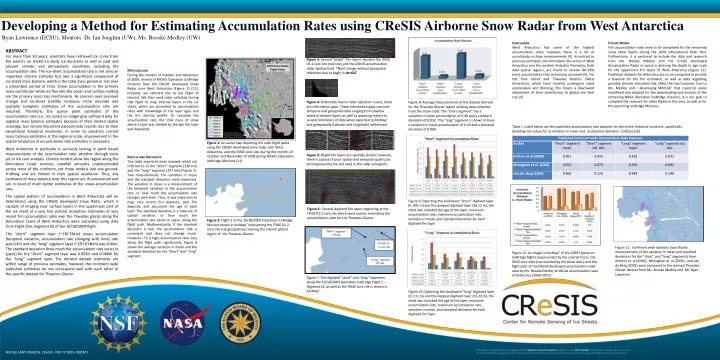
1. Developing a Method for Estimating Accumulation Rates using CReSIS Airborne Snow Radar from West Antarctica Ryan Lawrence (ECSU), Mentors: Dr. Ian Joughin (UW), Ms. Brooke Medley (UW) • Conclusion • West Antarctica has some of the highest accumulation rates; however, there is a lot of uncertainty in those measurements [4]. In contrast to previous estimates, the Amundsen Sea sector of West Antarctica and the western Antarctic Peninsula, both data sparse regions, are found to receive 80–96% more accumulation than previously assumed [4]. For the Pine Island and Thwaites Glaciers (West Antarctica), which have recently undergone rapid acceleration and thinning, this means a downward adjustment of their contribution to global sea level rise [4]. • Future Works • Firn accumulation rates need to be completed for the remaining snow radar flights during the 2009 International Polar Year. Furthermore, it is pertinent to include the data and research from Ms. Brooke Medley and the CreSIS developed Accumulation Radar to assist in deriving the depth to age scale for the uppermost firn layers of West Antarctica (Figure 12). Published datasets for Antarctica are to be compared to provide a baseline for the firn estimates, as well as data regarding possible climatic indicators that affect the mass balance. Due to Ms. Medley and I developing MATLAB® that could be easily modifieed and adapted for the downloading and analysis of the remaining NASA Operation IceBridge missions, it is our goal to complete the research for other flights in the area, as well as for the upcoming IceBridge Missions. ABSTRACT For more than 50 years, scientists have retrieved ice cores from the world's ice sheets to study ice dynamics as well as past and present climatic and atmospheric conditions, including the accumulation rate. The ice-sheet accumulation rate is not only an important climate indicator but also a significant component of ice-sheet mass balance, which is the total mass gained or lost over a prescribed period of time. Snow accumulation is the primary mass contributor while ice flux into the ocean and surface melting are the primary mass loss mechanisms. As concern over sea-level change and ice-sheet stability increases, more accurate and spatially complete estimates of the accumulation rate are required. Therefore, the sparse point estimates of the accumulation rate (i.e., ice cores) no longer give sufficient data for regional mass balance estimates because of their limited spatial coverage, but remain important paleoclimate records due to their exceptional temporal resolution. In order to constrain current mass balance estimates at the regional scale, improvement in the spatial resolution of accumulation rate estimates is necessary. West Antarctica in particular is seriously lacking in point based measurements of the accumulation rate, whether through snow pit or ice core analysis. Climate models show the region along the Amundsen Coast receives snowfall amounts unprecedented across most of the continent, yet these models lack any ground-truthing and are limited in their spatial resolution. Thus, any estimates of mass balance over this region are ill-constrained and are in need of much better estimates of the snow accumulation rate. The spatial pattern of accumulation in West Antarctica will be determined using the CReSIS developed Snow Radar, which is capable of imaging near surface layers in the uppermost part of the ice sheet at a very fine vertical resolution. Estimates of very recent firn accumulation rates over the Thwaites glacier along the Amundsen Coast of West Antarctica were calculated using data from Flight One, Segment 02 of the 10/18/2009 flight. The “short” segment layer (~130.76km) mean accumulation (temporal variation, accumulation rate changing with time) rate was 0.4m and the “long” segment layer (~297.874km) was 0.44m. The standard deviation (how much the accumulation rate varies in space) for the “short” segment layer was 0.052m and 0.068m for the “long” segment layer. The derived dataset estimates are within range of previous estimates; however, the continent wide published estimates do not correspond well with each other or the specific dataset for Thwaites Glacier. Figure 3: Several “bright” firn layers intersect the ITASE 01-2 core site (red line) and the CReSIS accumulation radar (yellow line). *Note: Image without geospatial reference due to begin in ArcGIS® • Methodology • During the months of October and November of 2009, several of NASA’s Operation IceBridge missions flew the CReSIS developed Snow Radar over West Antarctica (Figure 1) [11]; however, we selected one as our flight of interest. We then used radar collected during that flight to map internal layers in the ice sheet, which we converted to accumulation rates with knowledge of the layer ages and the firn density profile. To calculate the accumulation rate, the total mass of snow above a layer was divided by the age the layer was deposited. Figure 4: Potentially due to radar operation issues, there are information gaps. These information gaps can omit temporal and geospatial data ranging from shallow layers to deeper layers, as well as spanning meters to several kilometers of data when exported to ArcMap® and geospatially (latitude and longitude) referenced. Figure 8: Average measurements of the dataset derived for the Thwaites Glacier region utilizing data collected from the snow radar. The “short segment” has a variation in mean accumulation of 0.40 and a standard deviation of 0.052. The “long” segment is shown to have a variation in mean accumulation of 0.44 and a standard deviation of 0.069. Table I: Listed below are the published accumulation rate datasets for the entire Antarctic continent, specifically detailing the values for 1) variation in mean and 2) standard deviation [14][15] [16]. Figure 1: An aerial map depicting the sixth flight paths using the CReSIS developed snow radar over West Antarctica, and the ITASE core site, during the months of October and November of 2009 during NASA’s Operation IceBridge Missions [11]. Figure 5: Bright firn layers are spatially shown; however, there is a place of poor spatial and temporal quality (as encompassed by the red oval) in the radar echogram. • Results and Discussion • Two radar segments were mapped, which are referred to as the “short” segment (130 km) and the “long” segment (297 km) (Figure 7). Two measurements, the variation in mean and the standard deviation, were examined. The variation in mean is a measurement of the temporalvariation in the accumulation rate, or how much the accumulation rate changes with time. Thus, it was important to map very recent firn deposits, past firn deposits, and document the age of each layer. The standard deviation is a measure of spatial variation, or how much the accumulation rate varies in space, along the flight path. Mathematically,if the standard deviation is low, the accumulation rate is consistent and does not change much. However, if it is high, accumulation rates vary along the flight path significantly. Figure 8 shows the average variation in mean and the standard deviation for the “short” and “long” segment. Figure 9: Depicting the shallowest “short” digitized layer (0. 805 m) and the deepest digitized layer (36.12 m), the chart also included the age of the layer, minimum accumulation rate, maximum accumulation rate, variation in mean, and standard deviation for each digitized firn layer. Figure 6: Several digitized firn layers beginning at the ITASE 01-2 core site which were used in estimating the accumulation rates for the Thwaites Glacier. Figure 2: Flight 1 of the 10/18/2009 Operation IceBridge Mission shown in ArcMap® intersecting the ITASE 01-2 core site and geospatially covering the interior glacial region of the Thwaites Glacier. Figure 11: Continent wide datasets (specifically measurements of the variation in mean and standard deviations for the “short” and “long” segments) from Arthern et. al (2006), Monaghan et. al (2006) , and van de Berg (2005) were compared to the derived Thwaites Glacier dataset from Ms. Brooke Medley and Mr. Ryan Lawrence. Figure 12: An image in ArcMap® of the 2009 Operation IceBridge flights (represented by the colored lines), the ITASE core sites (represented by the black dots), and the flight path of the CReSIS developed accumulation radar used by Ms. Brooke Medley to derive accumulation rates of Antarctica (2009-2010). Figure 7: The digitized “short” and “long” segments along the 10/18/2009 Operation IceBridge Flight 1 - Segment 02, as well as the ITASE core site is shown in ArcMap®. Figure 10: Depicting the shallowest “long” digitized layer (0. 311 m) and the deepest digitized layer (52.24 m), the chart also included the age of the layer, minimum accumulation rate, maximum accumulation rate, variation in mean, and standard deviation for each digitized firn layer. NSF REU ANT-0944255: CReSIS - NSF FY 2005-108CM1