Download
1 / 19
200 likes | 358 Vues
Variational Data Assimilation in Coastal Ocean Problems with Instabilities Alexander Kurapov J. S. Allen, G. D. Egbert, R. N. Miller College of Oceanic and Atmospheric Sciences Oregon State University. With support from ONR Physical Oceanography Program Grant N00014-98-1-0043.

E N D
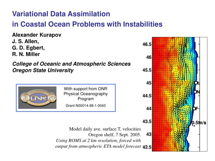
Variational Data Assimilation in Coastal Ocean Problems with Instabilities Alexander Kurapov J. S. Allen, G. D. Egbert, R. N. Miller College of Oceanic and Atmospheric Sciences Oregon State University With support from ONR Physical Oceanography Program Grant N00014-98-1-0043 Model daily ave. surface T, velocities Oregon shelf, 7 Sept. 2005. Using ROMS at 2 km resolution, forced with output from atmospheric ETA model forecast
Variational data assimilation is computationally expensive. Why use it? …Example using sequential Optimal Interpolation (OI): HF radars (Kosro) COAST data, summer 2001 Time-invariant gain matrix matrix matching observations to state vector Moorings (ADP, T, S: Levine, Kosro, Boyd) success… -Distant effect of assimilation of moored ADP currents (Kurapov et al., JGR, 2005a) -Effects of velocity assimilation on other fields of interest (JGR, 2005b) -Analysis of BML variability (JPO, 2005) and limitations…
OI: Correction term is present in the momentum equations Depth-ave, time-ave alongshore momentum term balance: OI corrects the ocean state, not forcing limited information on the source of model error OI assumes time-invariant forecast error covariance (Pf): DA no DA Satisfactory performance on average over the season, but possibly difficulties predicting events (instabilities, relaxation from upwelling to downwelling, etc.), when state-dependent covariance is needed. Snapshots of surf. velocity and density (<24.4 kg m-3), day 152, 2001: Less meandering in the data assimilation solution
Variational Data Assimilation: Theory Penalty Functional: J(u)= || Ini. error ||2 + || OB Cond. error ||2 + || Dynamical error ||2 + || Obs. error ||2 • Representer-based minimization algorithm (ref.: Chua and Bennett, OM, 2001): • Nontrivial covariances can be incorporated in J • Applicable both for strong-constraint (Dyn. error = 0) and weak-constraint cases • Involves search in a relatively small space spanned by representers • Provides error covariance in the prior and inverse solutions • Utilized in the emerging Inverse Ocean Modeling (IOM) System (Bennett et al.)
Details of the representer-based method: var(J) = 0 Euler-Lagrange Eqns. (nonlinear and coupled): where
Linearization and decoupling : Try to find a sequence of linearized solutions {un}, n=1,…,N {un} inverse solution To obtain un, the original ELE are linearized with respect to un-1 An optimal linear combination forcing the adjoint equation is obtained iteratively, solving the matrix-vector equation: prior (“Fwd”) solution of the linearized system representer matrix (K K) • Direct representer method (for small K). To obtain R, compute and sample (at data locations and times) K representer functions. To obtain a representer solution: • run the adjoint (AD) model, forced with • smooth the result with the model error covariance • run the tangent linear (TL) model Computational cost: (2 K + 1) N [equiv. fwd runs]
Indirect representer method (Egbert et al., 1994): • Use the conjugate gradient method to solve • To compute R b, where b is any vector: • run the AD model, forced with • smooth the result with the model error covariance, • run the TL model Preconditioning. Compute directly and sample a number of representer functions (obtain selected columns of R): Computational cost:<<(2 K + 1) N [equiv. fwd runs], depends on the number of degrees of freedom in the problem (the size of the domain, length of the run, assumed error covariances)
Implementation 1. Barotropic flow through the channel (Kuo jet) • (in collaboration with E. Di Lorenzo, A. Moore, H. Arango, et al.) • Use IROMS (in a version used originally for stability analyses): • correct initial conditions • direct representer method STEADY (SSH colored) Kuo jet: 2D, 100 x 400 km H=const=20 m, f=10-4 s-1 Periodic channel No forcing No dissipation PROPAGATING TO THE RIGHT (PERIOD 6.7 days) SSH mid-channel (NL ROMS): growth of instability is constrained days
Data assimilation experiment (with synthetic data): “True” (equilibrated wave): Prior: - symmetric jet, or - no flow Data: SSH or velocities, sampled from the true solution Goal: correct initial conditions Assimilation window: T=3-12 days Direct computation of representers. Does {un} converge to the inv. solution?
Dataless (Picard) iterations: No data. True controls (Ini. Cond.). Wrong background u0 (e.g., prior solution) Domain-averaged RMS error (surf. elevation) as a function of time: Picard Iterations: Convergence to truth for a limited period (comparable to the period of nonlinear oscillations) Data assimilation:convergence for a longer period of time Assimilatez at 40 locations on days 3, 6, 9, 12)
Choice of the IC error covariance affects convergence: IC penalty term: TL: includes IC errors in z, u, v Choices: 1. CIC=s2I singular un (Bennett, 2002) use Cgeos Cbell z RMS 2.Cbell: bell-shaped, independently for z, u, v u RMS 3.Cgeos: provide geostrophically balanced correction v RMS Lorenc (1981), Daley (1985) days (these cases: assim. z at t=3 d, prior= no flow)
Implementation 2. Forced-dissipative nearshore flows Alongshore currents over variable beach topography (Slinn et al. 2000) • In response to steady forcing, • steady flow, • equilibrated shear waves, • or “turbulent” regime, • depending on how large bottom friction is DA: correct forcing, initial, cross-shore boundary conditions Shown is Vorticity (NL ROMS, 2D, ADV_4C,biharmonic horiz. diff.) alongshore coord. (m)
Inverse model of choice: AKM TL and AD for shallow-water equations. Limited set of model options (straight periodic or OB channel, ADV_2C, harmonic horiz. diff., variable H) • Reasons to proceed with our TL&AD development: • Better understand how TL and AD are built in ROMS. • Clarify details of (and possibly suggest effective solutions for): • - time-stepping in the TL and AD • - inputs and outputs • 3. Interface with IOM (AKM has been incorporated in IOM) • 4. Address the issue of instabilities vs. variational DA in a simpler, 2D set-up
No background rhs arrays in TL or AD TL of time stepping momentum eqn.: Automatic Differentiation Tool / AKM
Inputs and outputs in TL and AD (AKM): - Avoid saving the AD solution every time step - Minimum (no) modifications to the code when using new data types Inputs: forcing, boundary values (sms_time, bry_time) NL, TL: interpolation Input: IC time Output: zeta, ubar, vbar every NHIS time steps u = [TL] f, length (u) length (f) [AD] = [TL]T y = [AD] v Input in ADM is a vector of the same length as output in TLM Output in ADM is a vector of the same length as input in TLM Outputs: corrections to forcing, boundary values (at sms_time, bry_time) AD: AD to interpolation Output: d(IC) time Input: a linear combination of data functionals (defined as a NetCDF file(s) of same format as a history file(s) in NL and TL, outside the code
Implementation of AKM in the forced-dissipative case: True solution: 250 x 200 m, Dx=2 m, periodic channel, NHIS=1 min, forcing is spatially variable, stationary in time (input: 2 identical fields at 0 and 60 min) time-ave, alongshore-ave u (m/s) Instant vorticity: 5 min 10 min 30 min 60 min v u time-ser. of v (m/s) time, min Prior: IC=0, forcing=0 (no flow)
Dataless (Picard) Iterations: no data, correct forcing, start with incorrect background (no flow) – does the series of linearized problems converge to truth? Time-series of u-RMS error: convergence for a limited time period Iter 5 Data assimilation:z, u, v every minute at 16 locations, T=30 min z-RMSE (m) v-RMSE u-RMSE (m/s) Total of 1200 obs. Computational requirements: Preconditioner: 24 rep. CGM: 20-30 iter. (for each linearized problem)
Possible approach 1: DA in a series of short (30 min) time windows, correct both forcing and IC in each window 2: Assume forcing is time-dependent Data assimilation, T=60 min (correcting time-invariant forcing): Mean current is restored, but meandering is not predicted deterministically Time-series of v-RMSE noconvergence in v Look for additional controls! 3: Open boundary control 4: Modify linearization scheme, step control
SUMMARY: • Clear advantages of using variational DA methods in problems of coastal and shelf circulation, to meet both scientific and operational needs • TL and AD ROMS (Kuo jet case): representer-based algorithm works for a period of time comparable to characteristic time scale of instabilities. Importance of using a dynamically based IC error covariance • AKM (nearshore, forced-dissipative case): experience building a TL&AD model. No background rhs arrays are needed. Clear definitions of inputs and outputs (no need to store the TL and AD solutions every time step; new data types can be incorporated without changes to TL&AD codes) • Possible approaches to overcome the problem of instabilities: look for additional controls (flow-forcing feedback; open boundary values)