Download
1 / 20
200 likes | 452 Vues
3rd LA PIETRA WEEK IN PROBABILITY Stochastic Models in Physics Firenze, June 23-27, 2008. SLE and conformal invariance for critical Ising model. Stanislav Smirnov. jointly with Dmitry Chelkak. 1D Ising model. 0 1 .…………………………………....... N N+1 ….…. + – + + + – – + – – + – + + ∙∙.

E N D
3rd LA PIETRA WEEK IN PROBABILITY Stochastic Models in Physics Firenze, June 23-27, 2008 SLE and conformal invariance for critical Ising model Stanislav Smirnov jointly with Dmitry Chelkak
1D Ising model 0 1 .…………………………………....... N N+1 ….…. +–+ + +– –+– –+–+ + ∙∙ Z=Σconf. x#{(+)(-)neighbors},P[conf.]~x #{(+)(-)} 0≤ x=e-J/kT ≤1. Let σ(0)=“+”. P[σ(N)=“+”] = ?
1D Ising model 0 1 .…………………………………....... N N+1 ….…. +–+ + +– –+– –+–+ + ∙∙ Z=Σconf. x#{(+)(-)neighbors},P[conf.]~x #{(+)(-)} 0≤ x=e-J/kT ≤1. Let σ(0)=“+”. P[σ(N)=“+”] = ? =½(1+yN), y=(1-x)/(1+x). Zn+1;σ(n+1)=“+” = Zn;σ(n)=“+” + xZn;σ(n)=“–” Zn+1;σ(n+1)=“–” = xZn;σ(n)=“+” + Zn;σ(n)=“–”
EXERCISE: Do the same in the magnetic field: P[configuration] ~ x #{(+)(-)} b #{(-)} , b>0, σ(0)=“+”. P[σ(N)=“+”]=?
EXERCISE: Do the same in the magnetic field: P[configuration] ~ x #{(+)(-)} b #{(-)} , b>0, σ(0)=“+”. P[σ(N)=“+”]=? EXERCISE:Let σ(0)=“+”= σ(N+M). P[σ(N)=“+”]=? 0 ...……………………….. N ..………................. N+M +–+ + +– –+ –+–+ +–+ CheckP[σ(N)=“+”] → ½ (if N/M→const ≠ 0,1). [Ising ’25]:NO PHASE TRANSITION AT X≠0 (1D)
2D (spin) Ising model Squares of two colors, representing spins +,– Nearby spins tend to be the same: P[conf.]~ x#{(+)(-)neighbors} [Peierls ‘36]:PHASE TRANSITION (2D) [Kramers-Wannier ’41]:
σ(boundary of (2N+1)x(2N+1)=“+”) P[σ (0)=“+”]=? P[ ]≤ xL/(1+xL) ≤ xL, L=Length of P[σ (0)=“–”] ≤ Σj=1,..,NΣL≥2j+2 3LxL ≤ (3x)4/(1-(3x)2)(1-3x) ≤ 1/6, if x ≤ 1/6.
2D: Phase transitionx→1 (T→∞) x=xcrit x→0 (T→0) (Dobrushin boundary conditions:the upper arc is blue, the lower is red)
2D Ising model at criticality is • considered a classical example of • conformal invariance in statistical • mechanics, which is used in • deriving many of its properties. • However, • No mathematical proof has ever been given. • Most of the physics arguments concern nice domains only or do not take boundary conditions into account, and thus only give evidence of the (weaker!) Mobius invariance of the scaling limit. • Only conformal invariance of correlations is usually discussed, we ultimately discuss the full picture.
Theorem 1 [Smirnov]. Critical spin-Ising and FK-Ising models on the square lattice have conformally invariant scaling limits as the lattice mesh → 0. Interfaces converge to SLE(3) and SLE(16/3), respectively (and corresponding loop soups). Theorem 2 [Chelkak-Smirnov]. The convergence holds true on arbitrary isoradial graphs (universality for these models).
P[conf.]~ Π<jk>:σ(j)≠σ(k) Xjk Xjk= tan(αjk/2) σ(j) αjk σ(k) Ising model on isoradial graphs:
Some earlier results: LERW → SLE(2)UST →SLE(8)Percolation → SLE(6) [Lawler-Schramm [Smirnov, 2001] -Werner, 2001]
(Spin) Ising model Conigurations: spins +/– P ~ x#{(+)(-)neighbors} = Π<jk>[(1-x)+xδs(j)=s(k)]
(Spin) Ising model Conigurations: spins +/– P ~ x#{(+)(-)neighbors} = Π<jk>[(1-x)+xδs(j)=s(k)] Expand, for each term prescribe an edge configuration: x : edge is open 1-x : edge is closed open edges connect the same spins (but not all!)
Edwards-Sokol covering ‘88 Conigurations: spins +/–, openedges connect the samespins (but not all of them!) P ~ (1-x)#openx#closed
Fortuin-Kasteleyn (random cluster) model ’72: Conigurations: spins +/–, openedges connect the samespins (but not all of them!) P ~ (1-x)#openx#closed Erase spins: Probability of edge configurations is ~ to (1-x)#openx#clos2#clusters or ((1-x)/x)#open2#clusters
Loop gas representation: Conigurations: dense loop collections. P ~ to ((1-x)/x)#open2#clusters or ((1-x)/2½x)#open2½#loops [ #loops – #open = 2#clusters+const ] Self-dual case: (1-x)/x=2½, i.e. X=1/(1+ 2½)
Spin, FK, Loop gas EXERCISE: Pspin[σ(j)=σ(k)] = (1+PFK[j↔k])/2 EXERCISE: Start with Q different spins (Potts model). Note: Loop gas is well-defined for all positive Q’s!
Outline: Introduction Discrete harmonic/holomorphic functions Holomorphic observables in the Ising model SLE and the interfaces in the Ising model Further developments We will discuss how to Find an discrete holomorphical observablewith a conformally invariant scaling limit Using one observable, construct (conformallyinvariant) scaling limits of a domain wall Possible further topics: Retrieve needed a priori estimates from the observable Construct the full scaling limit Generalize to isoradial graphs (universality) Perturbation p→pcrit — no conformal invariance