Download

1 / 31
320 likes | 505 Vues
Hough transform. Hough Transform. Introduced in 1962 by Paul Hough pronounced like “tough” according to http://www.citidel.org/bitstream/10117/1289/1/HoughTransform.html Detects lines. Has been generalized to other shapes as well. Handles noise. Handles partial occlusion.

E N D
Hough Transform • Introduced in 1962 by Paul Hough • pronounced like “tough” according to http://www.citidel.org/bitstream/10117/1289/1/HoughTransform.html • Detects lines. • Has been generalized to other shapes as well. • Handles noise. • Handles partial occlusion.
Problem: We process a gray image and create a binary version. Next, we wish to fit lines to the binary image. • from http://www.cs.uregina.ca/Links/class-info/425-nova/Lab4/
More examples • from http://www.cc.utah.edu/~asc10/improc/project4/README.html
Problem: We process a gray image and create a binary version. Next, we wish to fit lines to the binary image. • Slope-intercept equation of line: • where a is the slope (y/ x), and b is the y-intercept
Problem: We process a gray image and create a binary version. Next, we wish to fit lines to the binary image. • Slope-intercept: y=ax+b • We typically think of (x,y) as variables and (a,b) as constants. • Instead, let’s think of (a,b) as variables and (x,y) as constants. Rewritten: b=-xa+y • Note that this is also the equation of a line but in (a,b) space. • We can pass (infinitely) many lines at different angles through (x,y). As we do this, we’ll form a line in (a,b) space.
Passing many lines through an (x,y) point. • Figure by Anne Solberg
Figure by Anne Solberg. • Two points in (x,y)-space define a line. • However (if we pass infinitely many lines through each of these points), we obtain two different lines in (a,b)-space for each of these points.
Figure by Anne Solberg. • Two points in (x,y)-space define a line. • However (if we pass infinitely many lines through each of these points), we obtain two different lines in (a,b)-space for each of these points. • Then line between them in (x,y)-space gives rise to a point of intersection in (a,b)-space.
problem • (a,b)-space can’t be used in practice because vertical lines have infinite slope!
problem • (a,b)-space can’t be used in practice because vertical lines have infinite slope! • Solution: • Use polar coordinates. Lines are then represented by their angle (from the x-axis) and perpendicular distance from the origin, r. • All points on the same line will have the same (r,). • (figure from http://en.wikipedia.org/wiki/Hough_transform)
note • Each point in (x,y)-space gives rise to a sinusoid in (r,)-space. • But that’s OK. Lines in (x,y)-space will still give rise to intersections in (r,)-space.
Data structure • Use an accumulator matrix (2D histogram; call it A) of counts for (r,). • Voting algorithm. • We’ll get one vote for each point along the sinusoid. • Two votes at points of intersection of sinusoids (which denote lines in (x,y)-space. • More than two votes for multiple co-linear points (in (x,y)-space). • Then the points in (r,)-space with the most votes denote strong lines in (x,y)-space.
Data structure • Use an accumulator matrix (2D histogram; call it A) of counts for (r,). • Voting algorithm. • So we need to quantize the allowable values for r and . • For r, we can use all the integer values from 0 to the largest image diagonal distance. (We could use more as well. For example, we could multiply this value by 10 and get up to a resolution of 10ths.) • For , we can quantize to one degree increments, or we can use the same number as used for r.
algorithm • Let Q be the number of angles into which was quantized. • For each point, pi in P: • For each qi in Q • Assume that a line at angle =qi passes through pi. • Calculate r for this line • Increment A[r, ]. • The values in A that exceed some threshold (or the K greatest values in A) are the strongest lines. • What is the complexity of this algorithm?
algorithm • Let Q be the number of angles into which was quantized. • For each point, pi in P: • For each qi in Q • Assume that a line at angle =qi passes through pi. • Calculate r for this line • Increment A[r, ]. • The values in A that exceed some threshold (or the K greatest values in A) are the strongest lines. • What is the complexity of this algorithm? |P|*|Q| • But since Q is a constant that we determine, we can think of it as |P|.
Generalization to other shapes • y = ax + b can be written as ax + b - y = 0. • In general, f(x,a)=0, where x and a are vectors. • Consider the equation of a circle, (x-a)2 + (y-b) 2 = r2. • So our vector x above will be <x,y> and a will be <a,b,r> (3D). • Consider the equation of an ellipse, (x-h) 2/a2 + (y-k) 2/b2 = 1. • In this case, our vector x will again be <x,y> and a will be <h,k,a,b> (4D). • However, this only characterizes ellipses that are aligned with the axes. So in general, for ellipses we need 5D space, <h,k,a,b,>.
Ex. two points: • (r==10 && c==10) • (r==100 && c==10)
Ex. four points: • (r==75 && c==75) • (r==200 && c==200) • (r==300 && c==300) • (r==500 && c==500)
Let’s take a look at one with gimp. • This test has just two point, (200,200) and (500,500). • We see nothing (at 18% magnification)!
At 100% we can begin to see the sinusoids. • But we are only changing theta by 0.1 so between 0..2 Pi there are only 62 samples. • So the intersections “miss.” • So let’s try more samples.
Let’s try sampling in one degree increments (resulting in 360 samples). • Now we see intersections!
Let’s try sampling in one degree increments (resulting in 360 samples). • Now we see intersections! • And a look at the PGM file confirms that the max value is 2.
Let’s try sampling in one degree increments (resulting in 360 samples). • Now we see intersections! • But there appears to be two! Why?
Let’s try sampling in one degree increments (resulting in 360 samples). • Now we see intersections! • But there appears to be two! Why? • Because we are rotating around 360 when we only need 180.
Better! • But now I’m afraid that I might miss intersections due to undersampling. So let’s sample tenths or hundredths of a degree (instead of one degree increments).
But where are the most votes? • Not at the points of intersection! • Why? • Because many points along the real curve are mapping (repeatedly) so a single point in our array.
Solution(S)? • (Oversample.) As you trace along a sinusoid, keep track of the last point and don’t count repetitions. • easier to code • less reliable • (Undersample.) As you trace along a sinusoid, draw straight lines between pairs of points (and still disallowing repeats as in #1). • harder to code • more reliable
Moral of the story: Sometimes it’s better to play “connect the dots” than it is to oversample!