Download
1 / 17
170 likes | 391 Vues
Lecture 5 Hough transform and RANSAC. Slides by: David A. Forsyth Clark F. Olson. Further abstraction. Even after edge detection we may have more information than we want. How can we abstract this even further? Choose a parametric object to represent a set of pixels

E N D
Lecture 5Hough transform and RANSAC Slides by: David A. Forsyth Clark F. Olson
Further abstraction • Even after edge detection we may have more information than we want. • How can we abstract this even further? • Choose a parametric object to represent a set of pixels • Example: a line (or segment) can represent a set of edge pixels • Other possibilities include circles and complex structures
Fitting • After deciding what representation you are using, there are three main questions: • How many objects are there? • To which of the objects does each pixel belong (if any)? • What parameters best represents each of the objects?
Curve extraction • One way to extract curves is to link edge pixels together. • A junction (3-way intersection) indicates a break point. • Can fit curves with model (line, conic section, etc.) after extraction. • However, this doesn’t usually work that well: • Edges are broken by areas of low contrast • Junctions are often missed by edge detectors • Another bad idea: test all possible lines (or other shape).
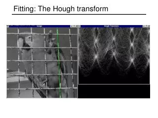
The Hough transform • The Hough transform is an important method for detecting structure (originally lines, but much more general). • The basic idea is to examine the parameter space for lines, rather than the image space, by mapping pixels in the image into the parameter space.
Line parameterizations A line is the set of points (x, y) such that: y = mx + b (slope-intercept) or (sin θ) x + (cos θ) y + ρ = 0 (rho-theta) (Two common ways to parameterize a line.)
The Hough transform • Different choices of m, b (or q, ρ) give different lines. • For any (x, y) there is a one parameter family of lines through this point. • Each point gets to vote for each line in the family; if there is a line that has lots of votes, that should be the line passing through the points
Example ρ y x pixels θ votes
Construct an array representing q, ρ. For each point, render the curve (q, ρ) into this array, adding one at each cell Mechanics of the Hough transform ρ y x pixels votes θ
Mechanics of the Hough transform • Issues: • How big should the cells be? • If too big, we can’t distinguish between different lines. • If too small, noise causes lines to be missed. • How many lines? • Count the peaks in the array. • Who belongs to which line? • Tag the votes, or post-process.
Example with noise ρ y x pixels votes θ
Random data ρ y x pixels votes θ
Hough transform algorithm Construct parameter space voting array (bins). For each edge pixel in image: Increment counter for each bin consistent with pixel. For each bin in voting array: Determine if sufficient votes exist (and local maximum). If so, output line.
Variations • Can use pairs of points to vote in parameter space • - Two points are consistent with only one line • Can use the edge gradient to reduce the number of bins consistent with an edge pixel • - One point plus orientation is consistent with only one line • Same ideas can be applied to many other structures: • - Circles • - Conic sections • - Arbitrary 2D shapes • - Three-dimensional objects
RANSAC (RANdomSAmple Consensus) is a useful algorithm using Monte Carlo sampling. Choose a small subset uniformly at random Fit the selected subset Anything else that is close to this fit is included Refit Do this many times and choose the best fits RANSAC
RANSAC • Issues: • How big a subset? • - Usually smallest possible • How many times? • - Often enough that we are likely to have a good line • How close is “close enough”? • - Depends on the problem