Download

1 / 85
880 likes | 1.12k Vues
Hedging Nonlinear Risk. Linear and Nonlinear Hedging. Linear hedging forwards and futures values are linearly related to the underlying risk factors Because linear combinations of normal random variables are also normally distributed, linear hedging maintains normal distributions

E N D
Linear and Nonlinear Hedging • Linear hedging forwards and futures values are linearly related to the underlying risk factors Because linear combinations of normal random variables are also normally distributed, linear hedging maintains normal distributions • Nonlinear hedging Options Since options can be replicated by dynamic trading of the underlying instruments, this also provides insights into the risks of active trading strategies Bahattin Buyuksahin, Celso Brunetti
Options: Notation St = current spot price of the asset in dollars Ft = current forward price of the asset K = exercise price of the option (also called strike price) ft = current value of the derivative instrument rt = domestic risk-free rate r*t = foreign risk free rate (also written as y: income produced by the asset) t = annual volatility of the rate of change (returns) in S = T – t = time to maturity For most options: ft = f(St , rt, r*t , t , K , ) Bahattin Buyuksahin, Celso Brunetti
Taylor Expansion • Option pricing is about finding f • Option hedging uses the partial derivatives • Risk management is about combining those with the movements in the risk factors • Remember: the Taylor approximation works only for small movements in the underlying risk factor Bahattin Buyuksahin, Celso Brunetti
A Simple Binomial Model • A stock price is currently $20 • In three months it will be either $22 or $18 Stock Price = $22 Stock price = $20 Stock Price = $18 Bahattin Buyuksahin, Celso Brunetti
A Call Option A 3-month call option on the stock has a strike price of 21. Stock Price = $22 Option Price = $1 Stock price = $20 Option Price=? Stock Price = $18 Option Price = $0 Bahattin Buyuksahin, Celso Brunetti
22D – 1 18D Setting Up a Riskless Portfolio • Consider the Portfolio: long position in Dshares of the stock and short 1 call option • Portfolio is riskless when 22D – 1 = 18D or D = 0.25 Bahattin Buyuksahin, Celso Brunetti
Valuing the Portfolio(Risk-Free Rate is 12%) • The riskless portfolio is: long 0.25 shares short 1 call option • The value of the portfolio in 3 months is 22*0.25 – 1 = 4.50=18*0.25 • The value of the portfolio today is 4.5e– 0.12*0.25 = 4.3670 Bahattin Buyuksahin, Celso Brunetti
Valuing the Option • The portfolio that is long 0.25 shares short 1 option is worth 4.367 today • The value of the portfolio today will be 20*0.25-f=4.367 where f represent option price today. • The value of the option is therefore f=5.000 – 4.367 f=0.633 Bahattin Buyuksahin, Celso Brunetti
uS0 ƒu S0 ƒ S0d ƒd Generalization • A derivative lasts for time T and is dependent on a stock Bahattin Buyuksahin, Celso Brunetti
Generalization(continued) • Consider the portfolio that is long D shares and short 1 derivative • The portfolio is riskless when S0uD – ƒu = S0dD – ƒd or S0 uD – ƒu S0– f S0dD – ƒd Bahattin Buyuksahin, Celso Brunetti
Generalization(continued) • Value of the portfolio at time T is S0uD – ƒu • Value of the portfolio today is (S0uD – ƒu )e–rT • Another expression for the portfolio value today is S0D – f • Hence ƒ = S0D – (S0uD – ƒu)e–rT Bahattin Buyuksahin, Celso Brunetti
Generalization(continued) • Substituting for D we obtain ƒ = [ p ƒu + (1 – p )ƒd ]e–rT where Bahattin Buyuksahin, Celso Brunetti
S0u ƒu S0 ƒ S0d ƒd Risk-Neutral Valuation • ƒ = [ p ƒu + (1 – p )ƒd ]e-rT • The variables p and (1– p ) can be interpreted as the risk-neutral probabilities of up and down movements • The value of a derivative is its expected payoff in a risk-neutral world discounted at the risk-free rate p (1– p ) Bahattin Buyuksahin, Celso Brunetti
Irrelevance of Stock’s Expected Return • When we are valuing an option in terms of the underlying stock the expected return on the stock is irrelevant • This is an example of a more general result stating that the expected return on the underlying asset in the real world is irrelevant Bahattin Buyuksahin, Celso Brunetti
Original Example Revisited S0u = 22 ƒu = 1 p • Since p is a risk-neutral probability • 20e0.12 *0.25 = 22p + 18(1 – p ); p = 0.6523 • Alternatively, we can use the formula S0 ƒ S0d = 18 ƒd = 0 (1– p ) Bahattin Buyuksahin, Celso Brunetti
S0u = 22 ƒu = 1 0.6523 S0 ƒ S0d = 18 ƒd = 0 0.3477 Valuing the Option The value of the option is e–0.12*0.25 [0.6523*1 + 0.3477*0] = 0.633 Bahattin Buyuksahin, Celso Brunetti
24.2 22 19.8 20 18 16.2 A Two-Step ExampleFigure 11.3, page 242 • Each time step is 3 months • K=21, r=12% Bahattin Buyuksahin, Celso Brunetti
Valuing a Call Option 24.2 3.2 D • Value at node B is e–0.12´0.25(0.6523´3.2 + 0.3477´0) = 2.0257 • Value at node A is e–0.12´0.25(0.6523´2.0257 + 0.3477´0) = 1.2823 22 B 19.8 0.0 20 1.2823 2.0257 A E 18 C 0.0 16.2 0.0 F Bahattin Buyuksahin, Celso Brunetti
72 0 D 60 B 48 4 50 4.1923 1.4147 A E 40 C 9.4636 32 20 F A Put Option Example K = 52, time step=1yr r = 5% Bahattin Buyuksahin, Celso Brunetti
72 0 D 60 B 48 4 50 5.0894 1.4147 A E 40 C 12.0 32 20 F What Happens When an Option is American Bahattin Buyuksahin, Celso Brunetti
Delta • Delta (D) is the ratio of the change in the price of a stock option to the change in the price of the underlying stock • The value of D varies from node to node Bahattin Buyuksahin, Celso Brunetti
Choosing u and d One way of matching the volatility is to set where s is the volatility and Dt is the length of the time step. This is the approach used by Cox, Ross, and Rubinstein Bahattin Buyuksahin, Celso Brunetti
The Probability of an Up Move Bahattin Buyuksahin, Celso Brunetti
The Stock Price Assumption • Consider a stock whose price is S • In a short period of time of length Dt, the return on the stock is normally distributed: where m is expected return and s is volatility Bahattin Buyuksahin, Celso Brunetti
The Lognormal Property • It follows from this assumption that • Since the logarithm of ST is normal, ST is lognormally distributed Bahattin Buyuksahin, Celso Brunetti
The Lognormal Distribution Bahattin Buyuksahin, Celso Brunetti
Continuously Compounded Return If x is the continuously compounded return Bahattin Buyuksahin, Celso Brunetti
The Expected Return • The expected value of the stock price is S0emT • The expected return on the stock is • m – s2/2 not m • This is because • are not the same Bahattin Buyuksahin, Celso Brunetti
m and m−s2/2 Suppose we have daily data for a period of several months • m is the average of the returns in each day [=E(DS/S)] • m−s2/2 is the expected return over the whole period covered by the data measured with continuous compounding (or daily compounding, which is almost the same) Bahattin Buyuksahin, Celso Brunetti
The Concepts Underlying Black-Scholes • The option price and the stock price depend on the same underlying source of uncertainty • We can form a portfolio consisting of the stock and the option which eliminates this source of uncertainty • The portfolio is instantaneously riskless and must instantaneously earn the risk-free rate • This leads to the Black-Scholes differential equation Bahattin Buyuksahin, Celso Brunetti
The Derivation of the Black-Scholes Differential Equation Bahattin Buyuksahin, Celso Brunetti
The Derivation of the Black-Scholes Differential Equation continued Bahattin Buyuksahin, Celso Brunetti
The Derivation of the Black-Scholes Differential Equation continued Bahattin Buyuksahin, Celso Brunetti
The Differential Equation • Any security whose price is dependent on the stock price satisfies the differential equation • The particular security being valued is determined by the boundary conditions of the differential equation • In a forward contract the boundary condition is ƒ = S – K when t =T • The solution to the equation is ƒ = S – K e–r (T – t ) Bahattin Buyuksahin, Celso Brunetti
The Black-Scholes Formulas Bahattin Buyuksahin, Celso Brunetti
The N(x) Function • N(x) is the probability that a normally distributed variable with a mean of zero and a standard deviation of 1 is less than x Bahattin Buyuksahin, Celso Brunetti
Properties of Black-Scholes Formula • As S0 becomes very large ctends to S0– Ke-rTand p tends to zero • As S0 becomes very small c tends to zero and p tends to Ke-rT– S0 Bahattin Buyuksahin, Celso Brunetti
Risk-Neutral Valuation • The variable m does not appear in the Black-Scholes equation • The equation is independent of all variables affected by risk preference • The solution to the differential equation is therefore the same in a risk-free world as it is in the real world • This leads to the principle of risk-neutral valuation Bahattin Buyuksahin, Celso Brunetti
Applying Risk-Neutral Valuation 1. Assume that the expected return from the stock price is the risk-free rate 2. Calculate the expected payoff from the option 3. Discount at the risk-free rate Bahattin Buyuksahin, Celso Brunetti
Valuing a Forward Contract with Risk-Neutral Valuation • Payoff is ST – K • Expected payoff in a risk-neutral world is S0erT –K • Present value of expected payoff is e-rT[S0erT –K]=S0– Ke-rT Bahattin Buyuksahin, Celso Brunetti
Implied Volatility • The implied volatility of an option is the volatility for which the Black-Scholes price equals the market price • There is a one-to-one correspondence between prices and implied volatilities • Traders and brokers often quote implied volatilities rather than dollar prices Bahattin Buyuksahin, Celso Brunetti
Option price Slope = D B Stock price A Delta • Delta (D) is the rate of change of the option price with respect to the underlying Bahattin Buyuksahin, Celso Brunetti
Delta Hedging • This involves maintaining a delta neutral portfolio • The delta of a European call on a non-dividend paying stock isN (d1) • The delta of a European put on the stock is N (d1) – 1 Bahattin Buyuksahin, Celso Brunetti
Delta Hedgingcontinued • The hedge position must be frequently rebalanced • Delta hedging a written option involves a “buy high, sell low” trading rule Bahattin Buyuksahin, Celso Brunetti
Delta • Key concept: The delta of an at-the-money call option is close to 0.5. Delta moves to 1 as the call goes deep in-the-money. It moves to 0 as the call goes deep out-of-the-money • Key concept: The delta of an at-the-money put option is close to -0.5. Delta moves to 1 as the put goes deep in-the-money. It moves to 0 as the put goes deep out-of-the-money Bahattin Buyuksahin, Celso Brunetti
Theta • Theta (Q) of a derivative (or portfolio of derivatives) is the rate of change of the value with respect to the passage of time • The theta of a call or put is usually negative. This means that, if time passes with the price of the underlying asset and its volatility remaining the same, the value of a long option declines Bahattin Buyuksahin, Celso Brunetti
Theta measures the sensitivity of an option to time Unlike other factors the movement in remaining maturity is perfectly predictable Time is not a risk factor is generally negative for long positions in both calls and puts the option loses value as time goes by At-the-money options lose a lot of value when the maturity is near For American options is always negative shorter-term American options are unambiguously less valuable than longer-term options Bahattin Buyuksahin, Celso Brunetti