Download
1 / 26
260 likes | 419 Vues
Emission Line Surveys Lecture 1. Mauro Giavalisco Space Telescope Science Institute University of Massachusetts, Amherst 1 1 From January 2007. Outline. Definitions Why emission lines Types of surveys and methodology Target surveys Blind surveys Sensitivity Narrow-band imaging

E N D
Emission Line SurveysLecture 1 Mauro Giavalisco Space Telescope Science Institute University of Massachusetts, Amherst1 1From January 2007
Outline • Definitions • Why emission lines • Types of surveys and methodology • Target surveys • Blind surveys • Sensitivity • Narrow-band imaging • Slit spectroscopy • Slitless spectroscopy • Observational techniques • Results from Emission Line Surveys • Historical notes • Discussion of recent and ongoing surveys • Methodology • Results • Future prospects
Disclaimer • We wrote these lectures from the point of view of the “observer” • They do not aim at providing a complete review of emission line surveys and their results • Rather, the choice of material is aimed at maximizing pedagogical value, illustrating current interesting problems, and at helping potential observers planning and designing their own emission line surveys • It also reflects our personal tastes and bias • Readers are strongly encouraged to do further, comparative research in any specific subject discussed here
Why Emission Line Surveys • To effectively look for a specific class of sources in some pre-assigned volumeof space and/or at some pre-assigned point in time • “effectively”: with high yield (low contamination) and in large numbers • Exploit the presence of emission line in the spectral energy distribution of most astrophysical sources • Traditional flux selection plus follow-up spectroscopy highly inefficient to cull special classes of sources from the general counts
Notations, Definitions, Reminders and World Model. I • Throughout these lectures, we use: • F: flux, in units of erg/s/cm2 • fn: flux density, in units of erg/s/cm2/Hz • fl: flux density, in units of erg/s/cm2/Å • fl = fn• |dn/dl| = fn• c/l2 • 1 Å = 10-8 cm • c = 2.9979 • 1010 cm/s
Notations, Definitions, Reminders and World Model. II • Throughout these lectures, we use: • L: luminosity, in units of erg/s • ln: luminosity density, in units of erg/s/Hz • ll: luminosity density, in units of erg/s/Å • fn = ln• (1+z)/ 4p• DL2(z) • fl = ll/ 4p• DL2(z) • (1+z) • F = L / 4p• DL2(z) • DL(z) = DL(z; H0, m, L) : luminosity distance • z is the redshift defined as z = a(t0)/a(t) – 1 • t is the cosmic time and t0 is the age of the universe
Notations, Definitions, Reminders and World Model. III • Throughout these lectures, we use: • AB magnitudes: • mAB = -2.5 • Log10(fn) - 48.595 • (Oke 1974; Oke & Gunn 1977) • ST magnitudes • mST = -2.5 • Log10(fl) - 21.1 • (Walsh 1995) • World Model (when needed): • H0 = 70 km/s/Mpc • m = 0.3; L = 0.7
CCD and near-IR Detectors • Most common devices used in emission line surveys • Photon counting devices: • DN = G • Ng • DN: Calibrated Data Number, I.e. what we read from the detector after calibrations • G: inverse gain • Ng: number of photons, in a finite wavelength interval Dl • Detectors add their own “signal” and noise: • DNobs = DN + K + e • K is removed during calibration (bias + d.c. + …) • e is a random variable with • <e> = 0 • < e2 > = ron2rms + d.c.2rms + … • Typical values: • [ron2rms]1/2 ~ a few (as low as ~1) to a few 10 e- /pix • [d.c.2rms]1/2 ~ 0.01 to a few e-/sec/pix • Let’s assume G=1 in the following
The Finite Resolution element • The smallest spatial scale or wavelength interval the instrumentation can resolve: • Spatial (PSF): the seeing (ground) or diffraction limit (space) • Good (bad) seeing: 0.6 (2) arcsec • HST resolution (V band): 0.03 arcsec • Depends on the size of the telescope, wavelength and… luck! • Poor image quality spreads photons over a large area, adds noise (2x seeing = 4x noise) • Spectroscopic (resolution): the spectral resolution element • Depends on the dispersion of the spectral element (prism, grism, grating) and on the slit aperture • If pixel size is well matched to resolution element (Nyquist sampling): FWHM (of PSF or LSF) covered by 4 pixels
S/N: Signal-to-Noise Ratio • Most important metric to asses sensitivity. • S/N in some finite wavelength interval Dl, either the passband width or the spectral resolution element • since we detect (count) photons, uncertainty on photon counting is simply dN = N1/2, and thus: • S/N = Sg / [Sg + Bg + N2g]1/2 • Sg : number of photons from source • Bg : number of photons from background • Ng : equivalent number of photons from additional sources of noise (typically detector)
Width of Emission Lines • The finite width of an emission line along the wavelength axis. • Commonly measured by the Full Width at Half Maximum (FWHM). For a gaussian line profile: • s ~ 0.425 • FWHM • The line width reflects the kinematics of the emission region (kinematics of the gas or of the individual sources in the case of integrated emission). If v is a measure of the velocity field within the emission region • Dl / l = Dv / c • If source is at redshift z, wavelengths are “stretched” by (1+z), thus observed FWHM and rest-frame FWHM related by: • FWHM(obs) = FWHM(rest) • (1+z)
Equivalent Width of Emission Lines • Metric to asses the strength of an emission line. • The width of a top-hat emission line of equal luminosity and peak value equal to the continuum at the line wavelength • It represents the wavelength range over which the continuum luminosity equals the line luminosity • Wl = L / ll = F / fl • Unaffected by extinction (line and continuum extinct by equal amount) • If source is at redshift z, wavelengths are “stretched” by (1+z), but luminosity (number of photons) is conserved. Thus, observed Wl and rest-frame Wl related by • Wl(obs) = Wl(rest) • (1+z)
How to Detect Emission Lines • Directly: observing the spectra of some class of candidates • Indirectly: comparing the photometry of the line through narrow-band passbands (on-band images) to that of the continuum through either narrow or broad-band passbands (off-band images)
Spectroscopy Lya z=5.65 Vanzella et al., in prep.
Unattenuated Spectrum Spectrum Attenuated by IGM B435 V606 z850 Finding galaxies at high-redshift: colorselection B435V606i775z850 • Color selection is very efficient in finding galaxies with specific spectral types in a pre-assigned redshift range • Wide variety of methods available, targeting a range of redshifts, galaxies’ SEDs: • Lyman and Balmer break (Steidel et al., GOODS) • BX/BM • (Adelberger et al., COSMOS) • DRG • (van Dokkum et al., GOODS) • BzK • (Daddi et al.) • Photo-z • (Mobasher et al) • Here, the case of • “Lyman-break galaxies” z~4