Download
1 / 54
540 likes | 548 Vues
Segmentation by fitting a model: Hough transform and least squares. T-11 Computer Vision University of Ioannina Christophoros Nikou. Images and slides from: James Hayes, Brown University, Computer Vision course

E N D
Segmentation by fitting a model: Hough transform and least squares T-11 Computer Vision University of Ioannina Christophoros Nikou Images and slides from: James Hayes, Brown University, Computer Vision course D. Forsyth and J. Ponce. Computer Vision: A Modern Approach, Prentice Hall, 2003. Computer Vision course by Svetlana Lazebnik, University of North Carolina at Chapel Hill. Computer Vision course by Kristen Grauman, University of Texas at Austin.
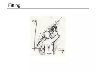
Fitting: motivation 9300 Harris Corners Pkwy, Charlotte, NC • We’ve learned how to detect edges, corners, blobs. Now what? • We would like to form a higher-level, more compact representation of the features in the image by grouping multiple features according to a simple model.
Fitting: motivation • Choose a parametric model to represent a set of features. simple model: circles simple model: lines complicated model: car Source: K. Grauman
Fitting: issues • Choose a parametric model to represent a set of features. • Membership criterion is not local • Can’t tell whether a point belongs to a given model just by looking at that point. • Three main questions: • What model represents this set of features best? • Which feature to which of several models? • How many models are there? • Computational complexity is important • It is infeasible to examine every possible set of parameters and every possible combination of features
Fitting: issues Case study: Line detection • Noise in the measured feature locations. • Extraneous data: clutter (outliers), multiple lines. • Missing data: occlusions.
Fitting: issues • If we know which points belong to the line, how do we find the “optimal” line parameters? • Least squares. • What if there are outliers? • Robust fitting, RANSAC. • What if there are many lines? • Voting methods: RANSAC, Hough transform. • What if we’re not even sure it’s a line? • Model selection.
Voting schemes • Let each feature vote for all the models that are compatible with it • Hopefully the noise features will not vote consistently for any single model • Missing data doesn’t matter as long as there are enough features remaining to agree on a good model
Hough transform • An early type of voting scheme. • General outline: • Discretize parameter space into bins • For each feature point in the image, put a vote in every bin in the parameter space that could have generated this point • Find bins that have the most votes Image space Hough parameter space P.V.C. Hough, Machine Analysis of Bubble Chamber Pictures, Proc. Int. Conf. High Energy Accelerators and Instrumentation, 1959
Hough transform • A line in the image corresponds to a point in Hough space Image space Hough parameter space Source: S. Seitz
Hough transform • What does a point (x0, y0) in the image space map to in the Hough space? Image space Hough parameter space
Hough transform • What does a point (x0, y0) in the image space map to in the Hough space? • Answer: the solutions of b = –x0m + y0 • This is a line in Hough space Image space Hough parameter space
Hough transform • Where is the line that contains both (x0, y0) and (x1, y1)? Image space Hough parameter space (x1, y1) (x0, y0) b = –x1m + y1
Hough transform • Where is the line that contains both (x0, y0) and (x1, y1)? • It is the intersection of the lines b = –x0m + y0 and b = –x1m + y1 Image space Hough parameter space (x1, y1) (x0, y0) b = –x1m + y1
Hough transform • Problems with the (m,b) space: • Unbounded parameter domain • Vertical lines require infinite m • Alternative: polar representation Each point will add a sinusoid in the (,) parameter space
Hough transform • A: intersection of curves corresponding to points 1, 3, 5. • B: intersection of curves corresponding to points 2, 3, 4. • Q, R and S show the reflective adjacency at the edges of the parameter space. They do not correspond to points.
Hough transform votes features • 20 points drawn from a line and the Hough transform. • The largest vote is 20.
Hough transform Square Circle • The four sides of the square get the most votes. • In the circle, all of the lines get two votes and the tangent lines get one vote.
Hough transform • Several lines
Hough transform • Random perturbation in [0, 0.05] of each point. • Peak gets fuzzy and hard to locate. • Max number of votes is now 6. features votes
Hough transform • Number of votes for a line of 20 points with increasing noise:
Hough transform • Random points: uniform noise can lead to spurious peaks in the accumulator array. Max votes = 4. features votes
Hough transform • As the level of uniform noise increases, the maximum number of votes increases too and makes the task difficult.
Practical details • Try to get rid of irrelevant features • Take only edge points with significant gradient magnitude. • Choose a good grid / discretization • Too coarse: large votes obtained when too many different lines correspond to a single bucket. • Too fine: miss lines because some points that are not exactly collinear cast votes for different buckets. • Increment also neighboring bins (smoothing in accumulator array).
Hough transform: Pros • Can deal with non-locality and occlusion. • Can detect multiple instances of a model in a single pass. • Some robustness to noise: noise points unlikely to contribute consistently to any single bin.
Hough transform: Cons • Complexity of search time increases exponentially with the number of model parameters. • Non-target shapes can produce spurious peaks in parameter space. • It’s hard to pick a good grid size.
3. Hough votes Edges Find peaks and post-process
Hough transform example http://ostatic.com/files/images/ss_hough.jpg
Least squares line fitting • Data: (x1, y1), …, (xn, yn) • Line equation: yi = mxi + b • Find (m, b) to minimize • Is there any problem with this formulation? • We will find the solution first and we will discuss it afterwards.
Least squares line fitting Least squares solution to XB=Y:
Least squares line fitting • Problems • Not rotation-invariant. • It measures the error of the vertical coordinate only. • Fails completely for vertical lines.
Total least squares • Distance between point P(xn, yn) and line(ε): ax+by+c=0: (ε): ax+by+c=0 Unit normal: N=(a, b) P(xi, yi) • We impose the constraint a2+b2=1 becauseλax+λby+λc=0is the same line.
Total least squares • Find the parameters of the line (a, b, c) that minimize the sum of squared perpendicular distances of each point from the line: subject to a2+b2=1. (ε): ax+by+c=0 Unit normal: N=(a, b) P(xi, yi)
Total least squares Substituting c into E(a,b,c) and introducing the constriant:
Total least squares which may be written in matrix-vector form:
Total least squares • The solution is the eigenvector of A corresponding to the smallest eigenvalue (minimization of E) of the covariance matrix. • The second eigenvalue (the largest) corresponds to a perpendicular direction.
Total least squares Covariance matrix N = (a, b)
Least squares for general curves • We would like to minimize the sum of squared geometric distances between the data points and the curve. (xi, yi) d((xi, yi), C) curve C
Least squares for conics • Equation of a 2D general conic:C(a, x) = a · x = ax2 + bxy + cy2 + dx + ey + f = 0, a = [a, b, c, d, e, f], x = [x2, xy, y2,x, y, 1] • Algebraic distance: C(a, x). • Algebraic distance minimization by linear least squares:
Least squares for conics • Least squares system: Da = 0 • Need constraint on a to prevent trivial solution • Discriminant: b2 – 4ac • Negative: ellipse • Zero: parabola • Positive: hyperbola • Minimizing squared algebraic distance subject to constraints leads also to a generalized eigenvalue problem. A. Fitzgibbon, M. Pilu, and R. Fisher, Direct least-squares fitting of ellipses, IEEE Transactions on Pattern Analysis and Machine Intelligence, 21(5), 476--480, May 1999 .
Recap: Two Common Optimization Problems Problem statement Solution Problem statement Solution (matlab)
Least squares (global) optimization Good • Clearly specified objective • Optimization is easy Bad • May not be what you want to optimize • Sensitive to outliers • Bad matches, extra points • Doesn’t allow you to get multiple good fits • Detecting multiple objects, lines, etc.
Who came from which line? • Assume we know how many lines there are - but which lines are they? • easy, if we know who came from which line • Three strategies • Incremental line fitting • K-means • Probabilistic (later!)
Incremental line fitting A really useful idea; it’s the easiest way to fit a set of lines to a curve.