Download
1 / 1
10 likes | 78 Vues
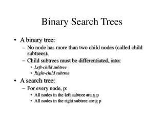
25. Root. 20. 30. 25. Depth = 0. 25. 10. 22. 28. 35. 20. 30. Depth = 1. 20. 30. Siblings. 5. 11. 21. Depth = 2. 10. 22. 28. 35. Leaves. Depth = 3. 5. 11. 21. Quantifying the dynamics of Binary Search Trees under combined insertions and deletions. .

E N D
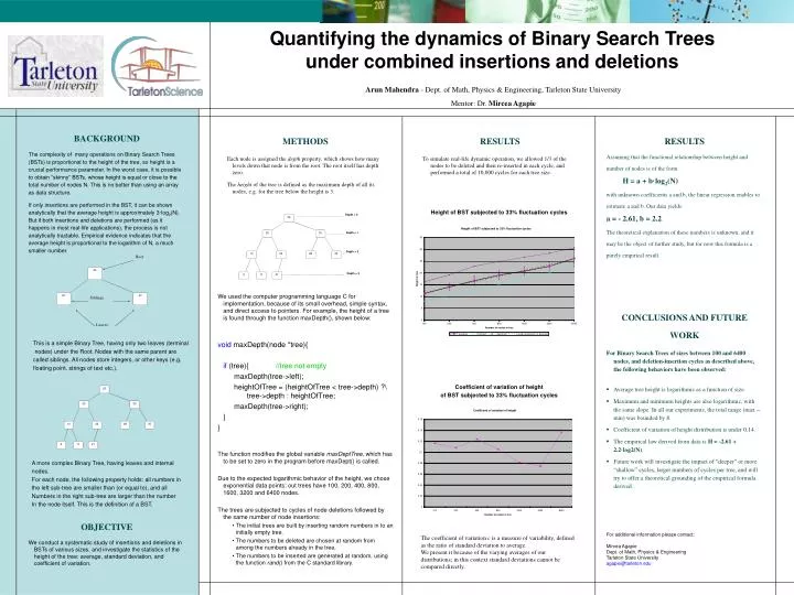
25 Root 20 30 25 Depth = 0 25 10 22 28 35 20 30 Depth = 1 20 30 Siblings 5 11 21 Depth = 2 10 22 28 35 Leaves Depth = 3 5 11 21 Quantifying the dynamics of Binary Search Treesunder combined insertions and deletions  Arun Mahendra - Dept. of Math, Physics & Engineering, Tarleton State University Mentor: Dr. Mircea Agapie METHODS Each node is assigned the depth property, which shows how many levels down that node is from the root. The root itself has depth zero. The height of the tree is defined as the maximum depth of all its nodes, e.g. for the tree below the height is 3. RESULTS To simulate real-life dynamic operation, we allowed 1/3 of the nodes to be deleted and then re-inserted in each cycle, and performed a total of 10,000 cycles for each tree size. RESULTS Assuming that the functional relationship between height and number of nodes is of the form H = a + b·log2(N) with unknown coefficients a and b, the linear regression enables to estimate a and b. Our data yields: a = - 2.61, b = 2.2. The theoretical explanation of these numbers is unknown, and it may be the object of further study, but for now this formula is a purely empirical result. BACKGROUND The complexity of many operations on Binary Search Trees (BSTs) is proportional to the height of the tree, so height is a crucial performance parameter. In the worst case, it is possible to obtain “skinny” BSTs, whose height is equal or close to the total number of nodes N. This is no better than using an array as data structure. If only insertions are performed in the BST, it can be shown analytically that the average height is approximately 3·log2(N). But if both insertions and deletions are performed (as it happens in most real-life applications), the process is not analytically tractable. Empirical evidence indicates that the average height is proportional to the logarithm of N, a much smaller number. Height of BST subjected to 33% fluctuation cycles We used the computer programming language C for implementation, because of its small overhead, simple syntax, and direct access to pointers. For example, the height of a tree is found through the function maxDepth(), shown below: void maxDepth(node *tree){ if (tree){ //tree not empty maxDepth(tree->left); heightOfTree = (heightOfTree < tree->depth) ?\ tree->depth : heightOfTree; maxDepth(tree->right); } } The function modifies the global variable maxDeptTree, which has to be set to zero in the program before maxDept() is called. Due to the expected logarithmic behavior of the height, we chose exponential data points: out trees have 100, 200, 400, 800, 1600, 3200 and 6400 nodes. The trees are subjected to cycles of node deletions followed by the same number of node insertions: • The initial trees are built by inserting random numbers in to an initially empty tree. • The numbers to be deleted are chosen at random from among the numbers already in the tree. • The numbers to be inserted are generated at random, using the function rand() from the C standard library. CONCLUSIONS AND FUTURE WORK For Binary Search Trees of sizes between 100 and 6400 nodes, and deletion-insertion cycles as described above, the following behaviors have been observed: • Average tree height is logarithmic as a function of size. • Maximum and minimum heights are also logarithmic, with the same slope. In all our experiments, the total range (max – min) was bounded by 8. • Coefficient of variation of height distribution is under 0.14. • The empirical law derived from data is H = -2.61 + 2.2·log2(N). • Future work will investigate the impact of “deeper” or more “shallow” cycles, larger numbers of cycles per tree, and will try to offer a theoretical grounding of the empirical formula derived. This is a simple Binary Tree, having only two leaves (terminal nodes) under the Root. Nodes with the same parent are called siblings. All nodes store integers, or other keys (e.g. floating point, strings of text etc.). Coefficient of variation of height of BST subjected to 33% fluctuation cycles A more complex Binary Tree, having leaves and internal nodes. For each node, the following property holds: all numbers in the left sub-tree are smaller than (or equal to), and all Numbers in the right sub-tree are larger than the number In the node itself. This is the definition of a BST. OBJECTIVE We conduct a systematic study of insertions and deletions in BSTs of various sizes, and investigate the statistics of the height of the tree: average, standard deviation, and coefficient of variation. For additional information please contact: Mircea Agapie Dept. of Math, Physics & Engineering Tarleton State University agapie@tarleton.edu The coefficient of variation c is a measure of variability, defined as the ratio of standard deviation to average. We present it because of the varying averages of our distributions; in this context standard deviations cannot be compared directly.