Download
1 / 40
400 likes | 553 Vues
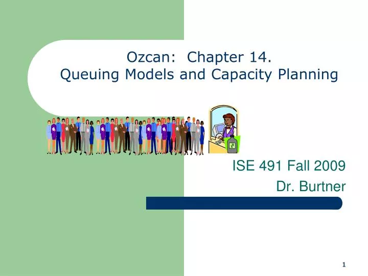
Ozcan: Chapter 14. Queuing Models and Capacity Planning. ISE 491 Fall 2009 Dr. Burtner. 1. Outline. Learning Objectives Queuing System Characteristics Population Source Servers Arrival Patterns Service Patterns Specific Queue Characteristics Measures of Queuing System Performance

E N D
Ozcan: Chapter 14. Queuing Models and Capacity Planning ISE 491 Fall 2009 Dr. Burtner 1
Outline • Learning Objectives • Queuing System Characteristics • Population Source • Servers • Arrival Patterns • Service Patterns • Specific Queue Characteristics • Measures of Queuing System Performance • Infinite Source-Models • Model Formulations • Single Server (M/M/1) • Multi Server (M/M/s>1) • Capacity Planning ISE 491 Fall 2009 Dr. Burtner Ch. 14 Ozcan
Learning Objectives Describe queuing systems and their potential applications in health care services. Describe various queuing model formulations. Analyze measures of queuing system performance Recognize queuing concepts and their relationship to capacity planning. 3 ISE 491 Fall 2009 Dr. Burtner Ch. 14 Ozcan
OZCAN: Figure 14.1 Queue Phenomenon ISE 491 Fall 2009 Dr. Burtner Ch. 14 Ozcan
Queuing Models • Develop a mathematical approach to the analysis of waiting lines • Weigh the cost of providing a given level of service capacity (i.e., shortening wait times) against the potential costs of having customers wait Reduce Wait Times Minimizing costs ISE 491 Fall 2009 Dr. Burtner Ch. 14 Ozcan
Costs • Waiting Costs • Salaries paid to employees while they wait for service (e.g., physicians waiting for an x-ray or test result) • Cost of waiting space • Loss of business due to wait • Balking customers • Reneging customers • Capacity Costs-- the cost of maintaining the ability to provide service ISE 491 Fall 2009 Dr. Burtner Ch. 14 Ozcan
Figure 14.2 Healthcare Service Capacity and Costs Total cost Cost of service capacity Cost Waiting line cost Optimum capacity Health care service capacity (servers) ISE 491 Fall 2009 Dr. Burtner Ch. 14 Ozcan
Queuing Model Characteristics • The population source • Infinite • Finite • The number of servers (channels) • Single line or multiple line • Single phase or multiple phase • Arrival and service patterns • Queue discipline (order of service) ISE 491 Fall 2009 Dr. Burtner Ch. 14 Ozcan
The Population Source • Finite source • Customer population where potential number of customers is limited • Infinite source • Customer arrivals are unrestricted • Customer arrivals exceed system capacity • Exists where service is unrestricted • The model used in our text ISE 491 Fall 2009 Dr. Burtner Ch. 14 Ozcan
Ozcan: Figure 14.3 Queuing Conceptualization of Flu Inoculations Facility Population (Patient Source) Queue (Waiting Line) Service Arrivals Exit Server ISE 491 Fall 2009 Dr. Burtner Ch. 14 Ozcan
The Number of Servers • Capacity is a function of the capacity of each server and the number of servers being used • Servers are also called channels • Systems can be single or multiple channel, and consist of phases • Most healthcare systems are multiple-line multiphase systems. ISE 491 Fall 2009 Dr. Burtner Ch. 14 Ozcan
Ozcan: Figure 14.4 Conceptualization of a Single-line, Multi-phase System Phase -1 Phase -2 Phase -3 Queue-1 Queue-2 Queue-3 Population Receptionist (server) Nurse (server) Physician (server) Arrivals Exit ISE 491 Fall 2009 Dr. Burtner Ch. 14 Ozcan
Ozcan: Figure 14.5 Multi-Line Queuing Systems Line-1 Queue Nurses Providing Inoculations Line-1 Patients Line-2 Line-3 Emergency Room Phase-2 Phase-3 Phase-1 Diagnostic Testing Physicians- Interventions Physicians- Initial Evaluation Queue-1 Queue-2 Queue-3 ISE 491 Fall 2009 Dr. Burtner Ch. 14 Ozcan
Arrival and Service Patterns • Both arrival and service patterns are random, thus causing waiting lines • Models assume that: • Customer arrival rate can be described by a Poisson distribution • Service time can be described by a negative exponential distribution ISE 491 Fall 2009 Dr. Burtner Ch. 14 Ozcan
OZCAN: Figure 14.7 Measures of Arrival Patterns Inter-arrival time 9:00pm 10:00pm ISE 491 Fall 2009 Dr. Burtner Ch. 14 Ozcan
Ozcan: Figure 14.8 Poisson Distribution .20 .15 .10 Probability .05 0 1 2 3 4 5 6 7 8 9 10 Patient arrivals per hour ISE 491 Fall 2009 Dr. Burtner Ch. 14 Ozcan
Exponential and Poisson Distributions If service time is exponential, then the service rate is Poisson. If the customer arrival rate is Poisson, then the inter-arrival time (i.e., the time between arrivals) is exponential. Example: If a lab processes 10 customers per hour (rate), the average service time is 6 minutes. If the arrival rate is 12 per hour, then the average time between arrivals is 5 minutes. Thus, service and arrival rates are described by the Poisson distribution and inter-arrival times and service times are described by a negative exponential distribution. ISE 491 Fall 2009 Dr. Burtner Ch. 14 Ozcan
Queue Behavior • Balking • Patients who arrive and see big lines (the flu shot example) may change their minds and not join the queue, but go elsewhere to obtain service; this is called balking. • Reneging • If patients join the queue and are dissatisfied with the waiting time, they may leave the queue; this is called reneging. ISE 491 Fall 2009 Dr. Burtner Ch. 14 Ozcan
QueueDiscipline • Queue discipline refers to the order in which patients are processed. • Adaptations in healthcare: • First-Come, First-Served (may be the most common practice) • Most Serious First-Served (emergency department triage system) • Shortest Processing Time, First Served (sometimes applied in operating room scheduling) ISE 491 Fall 2009 Dr. Burtner Ch. 14 Ozcan
System Metrics • Average number of patients waiting (in line or in system) • Average time patients wait (in line or in system) • System utilization (% of capacity utilized) • Implied costs of a given level of capacity and its related waiting line • Probability that an arriving patient will have to wait for service ISE 491 Fall 2009 Dr. Burtner Ch. 14 Ozcan
Tradeoffs Increases in system utilization are achieved at the expense of increases in both the length of the waiting line and the average waiting time. Most models assume that the system is in a steady state where average arrival and service rates are stable. Avg. Number or time waiting in line 0 System Utilization 100% ISE 491 Fall 2009 Dr. Burtner Ch. 14 Ozcan
Ozcan: Exhibit 14.1 Queuing Model Classification A: specification of arrival process, measured by inter-arrival time or arrival rate. M: negative exponential or Poisson distribution D: constant value K: Erlang distribution G: a general distribution with known mean and variance B: specification of service process, measured by inter-service time or service rate M: negative exponential or Poisson distribution D: constant value K: Erlang distribution G: a general distribution with known mean and variance C: specification of number of servers -- “s” D: specification of queue or the maximum numbers allowed in a queuing system E: specification of customer population ISE 491 Fall 2009 Dr. Burtner Ch. 14 Ozcan
Examples of Typical Infinite-Source Models • Single channel, M/M/s • Multiple channel, M/M/s>1, • where “s” designates the number of channels (servers). • These models assume steady state conditions and a Poisson arrival rate. ISE 491 Fall 2009 Dr. Burtner Ch. 14 Ozcan
OZCAN: Exhibit 14.2 Queuing Model Notation arrival rate service rate Lq average number of customers waiting for service L average number of customers in the system (waiting or being served) Wq average time customers wait in line W average time customers spend in the system system utilization 1/ service time Po probability of zero units in system Pn probability of n units in system ISE 491 Fall 2009 Dr. Burtner Ch. 14 Ozcan
InfiniteSourceModels:ModelFormulations Five key relationships that provide basis for queuing formulations and are common for all infinite-source models: 1.The average number of patients being served is the ratio of arrival to service rate. 2.The average number of patients in the system is the average number in line plus the average number being served. 3. The average time in line is the average number in line divided by the arrival rate. 4. The average time in the system is the sum of the time in line plus the service time. 5. System utilization is the ratio of arrival rate to service capacity. ISE 491 Fall 2009 Dr. Burtner Ch. 14 Ozcan
Single Channel, Poisson Arrival and Exponential Service Time (M/M/1). Performance Measures Single server or single team ISE 491 Fall 2009 Dr. Burtner Ch. 14 Ozcan
Single Channel, Poisson Arrival and Exponential Service Time (M/M/1). Example 14.1 A hospital is exploring the level of staffing needed for a booth in the local mall where they would test and provide information on diabetes. Previous experience has shown that, on average, every 15 minutes a new person approaches the booth. A nurse can complete testing and answering questions, on average, in 12 minutes. If there is a single nurse at the booth, calculate system performance measures including the probability of idle time and of 1 or 2 persons waiting in the queue. What happens to the utilization rate if another workstation and nurse are added to the unit? ISE 491 Fall 2009 Dr. Burtner Ch. 14 Ozcan
Example 14.1 Solution: 1 Arrival rate: λ = 1(hour) ÷ 15 = 60(minutes) ÷ 15 = 4 persons per hour. Service rate: μ = 1(hour) ÷ 12 = 60(minutes) ÷ 12 = 5 persons per hour. Average persons served at any given time Persons waiting in the queue Number of persons in the system Minutes of waiting time in the queue Minutes in the system (waiting and service) ISE 491 Fall 2009 Dr. Burtner Ch. 14 Ozcan
Example 14.1 Solution: 2 Arrival rate: λ = 1(hour) ÷ 15 = 60(minutes) ÷ 15 = 4 persons per hour. Service rate: μ = 1(hour) ÷ 12 = 60(minutes) ÷ 12 = 5 persons per hour. Calculate queue lengths of 0, 1, and 2 persons ISE 491 Fall 2009 Dr. Burtner Ch. 14 Ozcan
Example 14.1 Solution: 3 Current system utilization (s=1) System utilization with an additional nurse (s=2) System utilization decreases as we add more resources to it. ISE 491 Fall 2009 Dr. Burtner Ch. 14 Ozcan
FIG.14.10EXCEL SETUP AND SOLUTION TO THE DIABETES INFORMATION BOOTH PROBLEM ISE 491 Fall 2009 Dr. Burtner Ch. 14 Ozcan
Multi-Channel, Poisson Arrival and Exponential Service Time (M/M/s>1) ISE 491 Fall 2009 Dr. Burtner Ch. 14 Ozcan
Multi-Channel, Poisson Arrival and Exponential Service Time (M/M/s>1) Wa = the average time for an arrival not immediately served Pw = probability that an arrival will have to wait for service. ISE 491 Fall 2009 Dr. Burtner Ch. 14 Ozcan
Multi-Channel, Poisson Arrival and Exponential Service Time (M/M/s>1) Expanding on Example 14.1: The hospital found that among the elderly, this free service had gained popularity, and now, during week-day afternoons, arrivals occur on average every 6 minutes 40 seconds (or 6.67 minutes), making the effective arrival rate 9 per hour. To accommodate the demand, the booth is staffed with two nurses working during weekday afternoons at the same average service rate. What are the system performance measures for this situation? ISE 491 Fall 2009 Dr. Burtner Ch. 14 Ozcan
Multi-Channel, Poisson Arrival and Exponential Service Time (M/M/s>1) Solution: This is an M/M/2 queuing problem. The WinQSB solution provided in Exhibit 14.5 shows the 90% utilization. It is noteworthy that now each person has to wait on average one hour before they can be served by any of the nurses. On the basis of these results, the healthcare manager may consider expanding the booth further during those hours. ISE 491 Fall 2009 Dr. Burtner Ch. 14 Ozcan
Figure 14.12 System Performance Summary for Expanded Diabetes Information Booth with M/M/2 ISE 491 Fall 2009 Dr. Burtner Ch. 14 Ozcan
Figure 14.13 System Performance Summary for Expanded Diabetes Information Booth with M/M/3 ISE 491 Fall 2009 Dr. Burtner Ch. 14 Ozcan
Figure 14.14 Capacity Analysis ISE 491 Fall 2009 Dr. Burtner Ch. 14 Ozcan
Multi-Channel, Poisson Arrival and Exponential Service Time (M/M/s>1) Table 14.1 Summary Analysis for M/M/s Queue for Diabetes Information Booth ISE 491 Fall 2009 Dr. Burtner Ch. 14 Ozcan
Assumptions and Limitations • Steady state of arrival and service process • Independence of arrival and service is assumed • The number of servers is assumed fixed • Little ability to incorporate important exceptions to the general flow • Difficult to model all but simple processes ISE 491 Fall 2009 Dr. Burtner Ch. 14 Ozcan