Download

1 / 71
1.94k likes | 5.09k Vues
NON-IDEAL FLOW Residence Time Distribution. A. Sarath Babu. SCOPE: Design of non-ideal reactors Identify the possible deviations Measurement of RTD Quality of mixing Models for mixing Calculating the exit conversion in practical reactors.

E N D
NON-IDEAL FLOW Residence Time Distribution A. Sarath Babu
SCOPE: • Design of non-ideal reactors • Identify the possible deviations • Measurement of RTD • Quality of mixing • Models for mixing • Calculating the exit conversion in practical reactors
Practical reactor performance deviates from that of ideal reactor’s : • Packed bed reactor – Channeling • CSTR & Batch – Dead Zones, Bypass • PFR – deviation from plug flow – dispersion • Deviation in residence times of molecules • the longitudinal mixing caused by vortices and turbulence • Failure of impellers /mixing devices How to design the Practical reactor ?? What design equation to use ?? Approach: (1) Design ideal reactor (2) Account/correct for deviations
Deviations In an ideal CSTR, the reactant concentration is uniform throughout the vessel, while in a real stirred tank, the reactant concentration is relatively high at the point where the feed enters and low in the stagnant regions that develop in corners and behind baffles. In an ideal plug flow reactor, all reactant and product molecules at any given axial position move at the same rate in the direction of the bulk fluid flow. However, in a real plug flow reactor, fluid velocity profiles, turbulent mixing, and molecular diffusion cause molecules to move with changing speeds and in different directions. The deviations from ideal reactor conditions pose several problems in the design and analysis of reactors.
Possible Deviations from ideality: Short Circuiting or By-Pass – Reactant flows into the tank through the inlet and then directly goes out through the outlet without reacting if the inlet and outlet are close by or if there exists an easy route between the two.
Three concepts are generally used to describe the • deviations from ideality: • the distribution of residence times (RTD) • the quality of mixing • the model used to describe the system These concepts are regarded as characteristics of Mixing.
Analysis of non-ideal reactors is carried out in • three levels: • First Level: • Model the reactors as ideal and account or • correct for the deviations • Second Level: • Use of macro-mixing information (RTD) • Third Level: • Use of micro-mixing information – models for • fluid flow behavior
RTD Function: • Use of (RTD) in the analysis of non-ideal reactor • performance – Mac Mullin & Weber – 1935 • Dankwerts (1950) – organizational structure • Levenspiel & Bischoff, Himmelblau & Bischoff, • Wen & Fan, Shinner • In any reactor there is a distribution of • residence times • RTD effects the performance of the reactor • RTD is a characteristic of the mixing
Measurement of RTD RTD is measured experimentally by injecting an inert matrerial called tracer at t=0 and measuring its concentration at the exit as a function of time. Injection & Detection points should be very close to the reactor
ASSUMPTIONS 1. Constant flowrate u(l/min) and fluid density ρ(g/l). 2. Only one flowing phase. 3. Closed system input and output by bulk flow only (i.e., no diffusion across the system boundaries). 4. Flat velocity profiles at the inlet and outlet. 5. Linearity with respect to the tracer analysis, that is, the magnitude of the response at the outlet is directly proportional to the amount of tracer injected. 6. The tracer is completely conserved within the system and is identical to the process fluid in its flow and mixing behavior.
Desirable characteristics of the tracer: • non reactive species • easily detectable • should have physical properties similar to that of the reacting mixture • completely soluble in the mixture • should not adsorb on the walls • Its molecular diffusivity should be low and should be conserved • colored and radio active materials are the most widely used tracers
Types of tracer inputs: • Pulse input • Step input • Ramp input • Sinusoidal input Ramp input Pulse & Step inputs are most common
Pulse input of tracer In Pulse input N0 moles of tracer is injected in one shot and the effluent concentration is measured The amount of material that has spent an amount of time between t and t+t in the reactor: N = C(t) v t
The fraction of material that has spent an amount of time between t and t+t in the reactor: dN = C(t) v dt For pulse input
The age of an element is defined as the time elapsed since it entered the system.
Disadvantages of pulse input • injection must be done in a very short time • when the c-curve has a long tail, the analysis • can give rise to inaccuracies • amount of tracer used should be known • however, require very small amount of tracer • compared to step input
Step input of tracer In step input the conc. of tracer is kept at this level till the outlet conc. equals the inlet conc.
For step input: Disadvantages of Step input: • difficult to maintain a constant tracer conc. • RTD fn requires differentiation – can lead • to errors • large amount of tracer is required • need not know the amount of tracer used
Characteristics of the RTD: • E(t) is called the exit age distribution function • or RTD function • describes the amount of time molecules have • spent in the reactor
Cumulative age distribution function F(t): 28 Washout function W(t) = 1 - F(t):
Moments of RTD: What is the significance of these moments ??
If the distribution curve is only known at a number of discrete time values, ti, then the mean residence time is given by: This is what you use in the laboratory
Variance: • represents the square of the distribution spread and has the units of (time)2 • the greater the value of this moment, the greater the spread of the RTD • useful for matching experimental curves to one family of theoretical curves • Skewness: • the magnitude of this moment measures the extent that the distribution is skewed in one direction or other in reference to the mean
Space time vs. Mean residence time: • The Space time and Mean residence time would be • equal if the following two conditions are satisfied: • No density change • No backmixing In practical reactors the above two may not be valid and hence there will be a difference between them.
Normalized RTD function E(): What is the significance of E() ?? How does E(t) vs. t looks like for two ideal CSTRs of different sizes ?? How does E() vs. looks like for two ideal CSTRs of different sizes ??
Using the normalized RTD function, it is possible to compare the flow performance inside different reactors. If E() is used, all perfectly mixed CSTRs have numerically the same RTD. If E(t) is used, its numerical values can change for different CSTRs based on their sizes.
RTD for ideal CSTR: Material balance on tracer st to pulse input: in – out = accumulation 0 – vC = VdC/dt C(t) = C0 e-t/
RTD for PFR-CSTR series: For a pulse tracer input into CSTR the output would be : C(t) = C0e-t/s Then the outlet would be delayed by a time p at the outlet of the PFR. RTD for the system would be: 1/s p
If the pulse of tracer is introduced into the PFR, then the same pulse will appear at the entrance of the CSTR p seconds later. So the RTD for PFR-CSTR also would be similar to CSTR-PFR. Though RTD is same for both, performance is different
Remarks: • RTD is unique for a particular reactor • The reactor system need not be unique for a • given RTD • RTD alone may not be sufficient to analyze the • performance of non-ideal reactors • Along with RTD, a model for the flow behaviour • is required
Reactor modeling with RTD: • Zero parameter models: • Segregation model • Maximum mixedness model Micro-mixing models • II. One parameter models: • Tanks-in-series model • Dispersion model Macro-mixing models III. Two parameter models: