Download
1 / 64
640 likes | 1.72k Vues
3. Mixed production systems (pull/push and push/pull systems) ... It turns out that this law is valid for all production lines, not just those with zero variability. ...

E N D
Slide 1:Different Production Systems
There are three basic production control systems that are being practiced today 1. Push Systems (MRP, MRP II) 2. Pull Systems (Kanban, Conwip) 3. Mixed production systems (pull/push and push/pull systems)
Slide 2:Pull Systems of Production
In order to achieve successful quality, cost, and delivery ( customer satisfaction) in our manufacturing system, we must have three major systems in place: 1. Total Quality Control (or TQM) 2. Total Productive Maintenance; and 3. Just-in-time (JIT) production
Slide 3:Single Card Kanban Control
1 2 3 4 Material Flow Order Signal (pull) WIP Operation
Slide 4:CONWIP
1 2 3 4 Material Flow (push) Order Signal (pull) WIP Operation
Slide 5:Push Production Systems
Many companies today plan and control their manufacturing operations with information system based on MRP (materials requirements planning) or its successor, MRP II (manufacturing resource planning).
Slide 6:Push Production Systems
MRP in general is called a �push system� referring to the common image of in-process inventory being pushed from one work center to the next after completion of a work order. Push systems plan production based on forecasted demand in batches. Alternatively they are also called made to stock planning and control systems.
Slide 7:Push Production Systems
Slide 8:Pull Production Systems
Slide 9:CONWIP
CONWIP (CONstant Work In Process) is an alternative to Kanban where a new job is introduced into the line only if a job leaves the line. The system operates based on the principle that a departing job out of the line sends a production card back to the beginning of the line to authorize the release of a new job.
Slide 10:CONWIP
1 2 3 4 Material Flow (push) Order Signal (pull) WIP Operation
Slide 11:CONWIP
Estimating the card count (Little�s Formula) No. of Cards (WIP) = Demand x Cycle Time / Batch Size
Slide 12:CONWIP
From a modeling perspective, a CONWIP system looks like a closed queuing network, in which customers (jobs) never leave the system but instead circulate around the network indefinitely.
Slide 13:Kanban
The card signaling system used in Toyota, which is considered the classic pull system for JIT manufacturing. Common practice in pull production is to use standard-sized containers for holding and moving parts.
Slide 14:Necessary Conditions for Pull Production Systems
1. More planning and responsibility must reside in the hands of supervisors and worker teams. 2. The goal must be to produce to meet demand. 3. Focus and motivation is to reduce WIP. 4. TPM must be ongoing. 5. TQC must be ongoing (process monitor, SPC, source inspection, poka-yoke, and autonomation) 6. Setup times must be small (SMED) 7. Leveled/mixed production must be used. 8. Flow production must be implemented. 9. Cooperative work attitudes and team work should be ongoing.
Slide 15:Pull System as a Fixed Quantity Reorder System
The pull system is, in effect, a variant of the simple reorder-point system where a replenishment order is placed whenever inventory falls to a critical level.
Slide 16:Pull System as a Fixed Quantity Reorder System
The formula for re-order point is Re-order Point = Demand x (Lead-Time) +Safety Stock where, lead time (time between order and replenishment) = processing time + conveyance time
Slide 17:Pull System as a Fixed Quantity Reorder System
Example : Suppose demand for an item is 105 units per week; given a 5-day week, demand is 21 units per day. If production time is 0.1 day and the conveyance time is 0.4 days, what is the desired Re-order Point (ROP)? ROP = 21(0.1 + 0.4) = 10.5 ? 11 units Question: What happened to Safety Stock?
Slide 18:Pull System as a Fixed Quantity Reorder System
ROP estimated in terms of containers is Maximum # of full containers in a buffer= Demand x (Production time + Conveyance time) /Container size
Slide 19:Pull System as a Fixed Quantity Reorder System
Example: Same as the previous problem. Additional information is that each container holds three units. What is the number of containers (K) to order each time? Answer: K = 21(0.1 + 0.4) / 3 = 3.5 ? 4 containers
Slide 20:Pull System Container Size Determination
Containers size in a pull system is estimated by a rule of thumb, that a container should have the capacity to hold about 10% of the daily demand for the material it holds.
Slide 21:Single Card Kanban Control
1 2 3 4 Material Flow Order Signal (pull) WIP Operation
Kanban PostSlide 23:Kanban Card Calculations
The following simple formula is used in estimating the number of Kanban cards at a station: Parts consumed during 1 Kanban cycle No. of Kanbans = Number of parts per container Where Parts consumed = Average demand x (1+?) x (kanban cycle time) during 1 Kanban cycle
Slide 24:Simple Pull System
Example: Let unit processing time be 0.1 days, demand be 21 units per day and the container size be 3 units. Furthermore, the stations are next to each other so that conveyance time is assumed to be zero. What is the required number of cards for this Kanban system? K = (=21(0.1)/3 = 0.7 ? 1 card. Question: what happened to ? ?
Slide 25:Kanban Card Calculations Production Kanban with Constant Reorder Quantity
CT = Kanban Cycle Time = Kanban waiting time in receiving post + Kanban transfer time to ordering post + Kanban waiting time in ordering post + Lot processing cycle (internal setup + run time + in- process waiting time) +Container transfer time to final buffer +Container waiting time in the final buffer No. of Cards = Demand x (1+ ?) x Cycle Time/Parts in a container
Slide 26:Kanban Card Calculations Production Kanban with Constant Reorder Quantity
Example: Kanban waiting time in receiving post = 15 minutes Kanban transfer time to ordering post = 0.5 minutes Kanban waiting time in ordering post = 0.5 minutes Internal setup = 6 minutes Run time = 3 minutes/unit In-process waiting time) = 0 minute Container transfer time to final buffer = 0 minute Container waiting time in the final buffer = 17 minutes Container size = 3 units Determine the number of Kanban cards.
Slide 27:Kanban Card Calculations Production Kanban with Constant Reorder Quantity
Answer: Assume that 1 day is 480 minutes P = [15+0.5+0.5+(6+3(3)+0)+0+17]/480=0.1 day so K = 21(0.1)/3 = 0.7 ? 1 card. Question: What happened to ? ? How much safety factor did we build in by using K = 1 ? Answer: (1-0.7)/0.7 = 43%
Slide 28:Kanban Card Calculations Withdrawal Kanban with Constant Reorder Quantity
CT = Kanban Cycle Time = Kanban waiting time in receiving post + Kanban conveyance time to upstream buffer +Container conveyance time to downstream buffer +Container waiting time in downstream buffer No. of Cards = Demand x (1+ ?) x Cycle Time/Parts in a container
Slide 29:Kanban Card Calculations Withdrawal Kanban with Constant Reorder Quantity
Example: same data as before, this time Kanban waiting time in receiving post = 15 minutes Kanban conveyance time to upstream buffer = 10 minutes Container conveyance time to downstream buffer = 120 minutes Container waiting time in downstream buffer = 25 minutes What is the number of withdrawal cards needed? Answer: CT = 15+10+120+25 = 170 minutes = 0.354 days. K = 21(0.354) / 3 = 2.48 ? 3 cards. Question: How much safety factor did we have? Answer: (3 - 2.47)/2.48 = 20.1%
Slide 30:Kanban Card Calculations Supplier Kanban with Constant Order Cycle
CT = Kanban Cycle Time = Negotiated delay (lead time in hours) +Kanban conveyance time to supplier +Truck waiting time at supplier plant + Material conveyance time from supplier to company No. of Cards = Demand x (1+ ?) x Cycle Time/Parts in a container
Slide 31:Kanban Card Calculations Supplier Kanban with Constant Order Cycle
Example: same as before, in addition Negotiated delay (lead time in hours) =36 hours Kanban conveyance time to supplier = 4 hours Truck waiting time at supplier plant = 2 hours Material conveyance time from supplier to company = 4 hours What is the needed supplier kanban cards? CT = 36+4+2+4 = 46 hours = 1.5 days K = 21(1.5)/3 = 10.5 ? 11 cards
Slide 32:Kanban Card Calculations Signal Kanban for Lot Production
CT = Kanban Cycle Time = Kanban waiting time in receiving post + Kanban transfer time to ordering post + Kanban waiting time in ordering post + Lot processing cycle (internal setup + run time + in- process waiting time) +Container transfer time to final buffer No. of Cards = Demand x (1+ ?) x Cycle Time/Parts in a container
Slide 33:Factory Physics
Bottleneck rate = rate of the process center with the least long term capacity. Raw process time = sum of the long-term average process times of each workstation in the line. Critical WIP level The smallest level of WIP, where the maximum line productivity is achieved (at the maximum bottleneck rate).
Slide 34:Factory Physics
Throughput [TH]: the average output of a production process. Capacity of a station: upper limit in its throughput. Work in process (WIP): the inventory between the start and the end points of a production routing. All the products between, but not including the stock points. Cycle time (CT): average time from release of a job at the beginning of a routing to until it reaches an inventory point at the end of the routing. I.e., the time the part spends as WIP. It is more difficult to define this for the entire product.
Slide 35:Factory Physics Little's Law
The Little's law provides the fundamental relationship between WIP, cycle time (CT), and throughput (TH). Law 1. (Little's law) Throughput = WIP/Cycle Time or Cycle Time = WIP/Throughput It turns out that this law is valid for all production lines, not just those with zero variability. Moreover, it also applies to a single machine, a line or the entire factory. Some important uses of the Little's law follows.
Slide 36:Factory Physics Cycle time reduction
From Cycle Time = WIP/Throughput we deduce that reducing cycle time implies reducing WIP provided that the throughput remains the same. Hence large queues are a sign of opportunity to improve cycle time as well as WIP.
Slide 37:Factory Physics Law 2: (Best case performance)
The minimum cycle time (CTbest) for a given WIP level, w, is given by ? T0 , if w ? W0 CTbest = ? ? w/rb , otherwise The maximum throughput (THbest) for a given WIP level, w, is given by ? w/T0 , if w ? W0 THbest = ? ? rb , otherwise
Slide 38:Factory Physics Law 3: (Worst Case Performance)
The worst case cycle time for a given WIP level, w, is given by CTworst = wT0 The worst case throughput for a given WIP level, w, is given by THworst = 1/T0
Slide 39:Factory Physics Law 4 (Variability)
In steady state, increasing variability always increase average cycle times and WIP levels.
Slide 40:Factory Physics Law 5 (Variability placement)
Variability early in a routing has a larger impact on WIP and cycle times than equivalent variability later in the routing.
Slide 41:Factory Physics Law 6 (Move batches)
Cycle time over a segment of routing are roughly proportional to the move batch sizes used over that segment.
Slide 42:Factory Physics Law 7 (Process batches)
In stations with significant setups: 1. The minimum process batch size that yields a stable system may be greater than one. 2. As process batch size becomes large, cycle time grows proportionally with batch size. 3. If setup times are long enough, there will be a process batch size greater than one for which the average cycle time is minimized.
Slide 43:Factory Physics Law 8 (Pay me now or pay me later)
If you can not pay for variability reduction, you will pay in one or more of the following ways: 1. Long cycle times and high WIP levels. 2. Wasted capacity (low utilization of resources). 3. Lost throughput. 4. Unhappy customers.
Slide 44:Factory Physics Law 9 (Lead-time)
The manufacturing lead-time for a routing that yields a given service level is an increasing function of both the mean and variance of the cycle time of the routing.
Slide 45:Factory Physics Law 10 (CONWIP Efficiency)
For a given level of throughput, a push system will have more WIP on average than an equivalent CONWIP system. Corollary: For a given level of throughput, a push system will have longer average cycle times than an equivalent CONWIP system.
Slide 46:Factory Physics Law 11 (CONWIP robustness)
A CONWIP system is more robust to errors in WIP level than a pure push system is to errors in release rate.
Slide 47:Drum-Buffer-Rope (DBR) Technique
The DBR technique is first used in the OPT software developed by Eliyahu Goldratt, the father of the TOC. The main idea of DBR is based on bottleneck scheduling and the Theory of Constraint (TOC). The goal is to schedule the bottleneck for full utilization and subordinate the rest of the system to the needs of the bottleneck.
Slide 48:Drum-Buffer-Rope (DBR) Technique
One way to insure the continuous operation of the bottleneck is to use a CONWIP mechanism from the beginning of the line, up to and including the bottleneck (the pull side). Push the material downstream once it passes the bottleneck (the push side). Therefore, the DBR system is a mixed pull/push control system.
Slide 49:Drum-Buffer-Rope (DBR) Technique
Each order is scheduled to depart the bottleneck at such time that, if unimpeded from there on, will arrive at the customer�s hand �just in time�. All planned orders with known due dates are scheduled to depart from the bottleneck as described above by using the following formula: depart time = order due date - (sum of all remaining operations after the bottleneck)
Slide 50:Drum-Buffer-Rope (DBR) Technique
In order to schedule the jobs following the bottleneck, they are made available to the downstream operation immediately (i.e., pushed). This pushing is continued until each jobs earliest arrival times to downstream stations are calculated. Once these times are at hand, the process then orders the jobs on those machines by using single machine scheduling heuristic with earliest due date criterion.
Slide 51:Drum-Buffer-Rope (DBR) Technique
If during this ordering phase a job is delayed to depart a downstream machine (will cause a delay in fulfilling the order on time), yet another heuristic is used to reschedule that job on the bottleneck and the upstream operations, with the hope of delivering it to the customer on time. If a successful solution can not be found this way, then either the job is scheduled for overtime, or alternate routing is sought for for resolving the conflict.
Slide 52:Drum-Buffer-Rope (DBR) Technique
The processes prior to the bottleneck (upstream) are scheduled moving one machine at a time upstream from the bottleneck. The idea here is to schedule the jobs to arrive at the bottleneck �just in time� First the departure time from the machine just prior to the bottleneck is calculated. Note that we do know the scheduled depart time of the job from the bottleneck. Therefore, desired arrival to bottleneck = desired departure - processing time at the bottleneck = desired departure from the process just prior to the bottleneck
Slide 53:Drum-Buffer-Rope (DBR) Technique
This process is applied to all jobs. Similar to the bottleneck the desired arrival times are calculated by using desired arrival = desired departure - processing time = desired departure from the process just prior (upstream) to this operation Once the arrival times are at hand, again, one machine sequencing heuristic is used for scheduling the jobs on this machine. This process continues until all jobs are scheduled on all machines.
Slide 54:Drum-Buffer-Rope (DBR) Technique
This is also called infinite capacity planning in MRP terminology and also used similarly in i2 Technology�s famous Factory Planner (FP) software. Once the first machine is scheduled, this provides us with the desired arrival time of the raw material to support the just established schedule. According to this first machine start schedule, we then look at on hand and on order inventories to see if we can support the calculated schedule. If, for some jobs there is no raw material, then they should be ordered to arrive �just in time�. This is the �supply-chain-planning� phase of the DBR.
Slide 55:Drum-Buffer-Rope (DBR) Technique
The hardest part of the DBR is to convert the infinite capacity plan into finite capacity plan. This is not a small task. The problem, mathematically speaking, is a very difficult problem to solve. Let alone to find the optimal solution, it is sometimes impossible to find a feasible solution which satisfies all capacity constraints. Several heuristic procedures have also been suggested to find a good feasible solution. However, those heuristics can not guarantee a feasible solution even if there exists one.
Slide 56:Drum-Buffer-Rope (DBR) Technique
To protect the bottleneck from random fluctuations in process times, setup times and other unforeseen variability, a buffer time is established in front of the bottleneck machine. This time buffer protects the bottleneck by bringing the jobs to the bottleneck buffer by W time units earlier than needed so that the bottleneck will never starve for jobs. Here, W is the time buffer for the bottleneck. Its size depends on how much protection is desired to keep the bottleneck from running out of work.
Slide 57:Drum-Buffer-Rope (DBR) Technique
Let Lj represent the sum of processing times of all operations for job j before the bottleneck, and W be the desired time buffer. Since (j-1) jobs must go through the bottleneck before job j can be scheduled, we can write the desired relation as Lj + W ? ? (bi) Here, bi is the processing time of job I on the bottleneck operation.
Slide 58:Drum-Buffer-Rope (DBR) Technique
The advantage of the DBR technique is its ability to provide a means for supply chain planning. Furthermore, by using a pull system upstream from the bottleneck, the WIP is also controlled. The cycle time is reduced significantly since the material is ordered �just in time.� The production system is utilized to its fullest potential by insuring that jobs are always available for the bottleneck. Job-shop environment can also be scheduled by using the DBR technique.
Slide 59:Supply Chain Planning
Lean manufacturing philosophy recognizes that to acquire the best purchased items, it is often necessary to work with suppliers to make them the best. This means joint problem solving, practicing quality at the source, and exchanging information. This simply means establishing partnerships with your suppliers.
Slide 60:Supply Chain Planning
Slide 61:SUPPLIER FOCUS
Supplier focus is now recognized by WCM companies for increasing competitiveness. Suppliers are no longer �important� to success, they are critical to success.
Slide 62:SUPPLIER FOCUS
In essence, when customers and suppliers work together to reduce the waste and inefficiencies in design, manufacturing and logistics, the resulting partnership provides significant improvements that increase the competitive strength of each member.
Slide 63:Who is Your Supplier?
Your vendor Another facility within the company Another department within the plant Another process in the plant The employee right next to you providing your incoming material
Slide 64:New Form of Supplier Relationship
From supplier�s point of view, manufacturers are customers. Suppliers should guarantee quality, delivery and cost (QDC) to the manufacturers.
Slide 65:New Form of Supplier Relationship
In the delivery area, frequent, small lot, on-time deliveries should be targeted in order to make manufacturer-supplier linkages tighter. This can be achieved by establishing a pull (Kanban) system between the two parties and within each plant.
Slide 66:New Form of Supplier Relationship
In the quality area, the idea of �quality at the source� should be practiced as much as possible. Lean manufacturing and one piece flow should be practiced to the fullest extent. Use of Poka Yoke and SPC should be encouraged to the fullest extend. Help train your suppliers to start and travel on the Lean Manufacturing Journey.
Slide 67:New Form of Supplier Relationship
More and more manufacturers are requiring their suppliers to guarantee six-sigma quality, which becomes exceedingly difficult in the �push� or �batch� manufacturing world. This is another reason manufacturers are demanding their suppliers to become lean by turning into one piece flow cellular manufacturing systems with 100% inspection.
Slide 68:New Form of Supplier Relationship
The most dependable, cooperative suppliers should be identified and a close working relationship should be developed functioning as an �extended factory� from the manufacturer�s point of view. Having dedicated suppliers for production of certain parts is just like arranging machines for a dedicated material flow within a plant.
Slide 69:New Form of Supplier Relationship
More and more suppliers are getting closer to the manufacturers for improved communication, logistics, and reduced cost.
Slide 70:Vendor Selection and Certification
The entire process of achieving certification as a quality vendor is focused on building excellence in one�s manufacturing operations. The basis for evaluating performance and one�s current market position can be categorized into six elements:
Slide 71:Elements of Vendor Certification
Management systems Design, specifications, and change control Incoming purchased materials In-process operations and practices Finished goods Measurement and test systems
Slide 72:Elements of Vendor Certification Management Systems
Top management�s commitment, leadership and adherence to policy of Lean manufacturing and continuous quality improvement A quality manual (and plan?) for processes and procedures Employee education and training programs to support LM and TQ. An emphasis on quality systems for defect prevention A program for annual quality improvement (AQI) for the elimination of waste Statistical methods for problem identification and problem solving
Slide 73:Elements of Vendor Certification Management Systems (cont�d)
Documentation control of process requirements and specifications An organizational structure for fostering participative quality management A formal program for cost of quality The internal quality system audit
Slide 74:Elements of Vendor Certification Design Specifications and change control
System for defining and communicating a customer�s quality requirements into critical final-product control specifications Procedures to perform process capability for new product development Design review procedures Procedure for making customer and design review changes FMEA analysis performed for new product designs Print and engineering change control system System to distribute and communicate design changes
Slide 75:Elements of Vendor Certification Design Specifications and change control (cont�d)
System for process improvement and design revisions System for new-job startup process and documentation control System for product identification and lot traceability to the design level.
Slide 76:Elements of Vendor Certification Incoming Purchased Material
Assessment of supplier�s capability Qualification of supplier Certification of suppliers Receiving inspection instructions and documentation, with feedback for any problems Formal program for initiating, documenting, and implementing corrective actions with preventative measures Identification, isolation and disposition of nonconforming material
Slide 77:Elements of Vendor Certification Incoming Purchased Material (cont�d)
Reinspection and traceability of reworked parts Material planning, scheduling and job release control system Material storage control system for purchased components and supplies.
Slide 78:Elements of Vendor Certification In-Process Operations, Control, Practices
Process sheets and standard work instructions of each operation of each part, incorporating visual information where possible Knowledgeable and involved operators in Lean manufacturing, Kaizen and TQM. Setup instruction sheets for all equipment Instruction sheets for first- and last- piece inspection and in process inspection. Work flow and material identification and control
Slide 79:Elements of Vendor Certification In-Process Operations, Control, Practices (cont�d)
Inspection, scrap audit reports, and feedback control Customer return and rework procedures SPC and corrective actions Procedures for performing, documenting and distributing process-capability analysis Total preventative management (TPM) program in place.
Slide 80:Elements of Vendor Certification Finished goods
Material storage control system (FIFO?) Packaging and handling instructions Material distribution control (test, verify, record) Proper storage facility for quality preservation Final inspection and control at shipping Audit history and tracking of product quality
Slide 81:Elements of Vendor Certification Measurement and Test Systems
Gauge control program (incoming, in-process, final) Calibration schedule and records for all measurement and test equipment Traceability and conformance to national and international standards Deterioration tracking and maintenance program (fixtures, tooling, molds, patterns, etc.)
Slide 82:Elements of Vendor Certification
The list of elements above, in essence, provides a means to objectively evaluate the effectiveness of the quality systems/procedures and performance/adherence present in a manufacturing organization This evaluation, in turn, provides a basis for decision making, corrective actions, and ongoing quality improvement.
Slide 83:Supplier Lead Times
Vendors are continuously pressured by their customers for more frequent deliveries and shorter lead times Particularly those manufacturers which have advanced significantly along the lean manufacturing journey and converted into Kanban manufacturing control system are expecting more frequent deliveries just in time. Often several times a day and smaller quantities. If the vendor is not already into the lean manufacturing journey, they can satisfy these demands only at the expense of excess inventories.
Slide 84:Supplier Lead Times
Excess inventories and build to stock environment always increases manufacturing cost and compromises quality Larger lot production causes longer cycle times and thus longer lead times for promise to customers. Longer lead times, higher inventories, lower quality and increased manufacturing costs often leads to lost customer orders and abandonment by the customers In order to remain competitive we must become lean. Lean manufacturing is the key to staying competitive and winning more contracts, more profits, and growth.
Slide 85:Goal in Supplier Relations
Become a lean manufacturer and help transform your customers and vendors along your supply chain to become lean as well. This will require providing necessary technical know-how to your supply chain partners through company sponsored workshops, pilot projects and visits to help speed up their journey into lean manufacturing.