Download
1 / 53
530 likes | 775 Vues
Scientific Computing with Radial Basis Functions. C.S. Chen Department of Mathematics University of Southern Mississippi U.S.A. PURPOSE OF THE LECTURE.

E N D
Scientific Computing with Radial Basis Functions C.S. Chen Department of Mathematics University of Southern Mississippi U.S.A.
PURPOSE OF THE LECTURE TO SHOW HOW RADIAL BASIS FUNCTIONS (RBFs) CAN BE USED TO PROVIDE 'MESH-FREE' METHODS FOR THE NUMERICAL SOLUTION OF PARTIAL DIFFERENTIAL EQUATIONS.
MESHLESS METHOD MESH METHOD
Advantages of Meshless Methods • It requires neither domain nor surface discretization. • The formulation is similar for 2D and 3D problems. • It does not involve numerical integration. • Ease of learning. • Ease of coding. • Cost effectiveness due to the man-power reduction involved for the meshing.
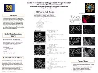
Radial Basis Functions Linear: Cubic: Multiquadrics: Polyharmonic Spines: Gaussian:
Compactly Supported RBFs • References • Z. Wu, Multivariate compactly supported positive definite radial • functions, Adv. Comput. Math., 4, pp. 283-292, 1995. • R. Schaback, Creating surfaces from scattered data using radial basis • functions, in Mathematical Methods for Curves and Surface, • eds. M. Dahlen, T. Lyche and L. Schumaker, Vanderbilt Univ. Press, • Nashville, pp. 477-496, 1995 • W. Wendland, Piecewise polynomial, positive definite and compactly • supported RBFs of minumal degree, Adv. Comput. Math., 4, pp 389- • 396, 1995.
Wendland’s CS-RBFs Define For d=1, For d=2, 3, For
Globally Supported RBFs =1+r
Surface Reconstruction Scheme Assume that To approximate f by we usually require fitting the given of pairwise distinct centres with the imposed data set conditions The linear system is well-posed if the interpolation matrix is non-singular
Meshless Method I Kansa’s Method or RBF Collocation Method
RBF Collocation Method (Kansa’s Method) Consider the Poisson’s equation (1) (2) We approximate u by û by assuming (3) where
(4) (5) By substituting (3), (5) into (1)-(2), we have (6) (7) can be obtained by solving NN system (6)-(7).
W W
For parabolic problems such as heat equation, we have (8) where t is the time step, and un and un+1 are the solutions at time tn=n t and tn+1=(n+1) t. Similar to elliptic problems, we assume (9)
Substituting (9) into (8) and (2), we have Notice that
Example I where RBFs: MQ, c = 0.8; i.e., Grid points: 19x19 Maximum error: 8.703E-5
Example II (Rotating Cone) Exact solution: where t = 0.01, t [0, 2] Maximum norm error = 0.001165 with c = 0.2 (MQ).
Approximate Sol. by Kansa’s Method (Rotating Cone) t=0.5 t=0.75 t=1.25 t=1.0
Maximum Error Norm by Kansa’s Method (Rotating Cone) t=0.75 t=0.5 t=1.0 t=1.25
Example III (Burgers’ Equation) Exact Solution t = 0.01, t [0, 1.25], = 0.05 Maximum norm error = 0.0719 with c = 0.2 (MQ).
Approximate Sol. of Kansa’s Method – Burger’s Equation t=0.75 t=0.5 t=1.0 t=1.25
Maximum Norm Error of Kansa’s Method t=0.75 t=0.5 t=1.0 t=1.25
CFD Example with the Kansa’s Method: Natural Convection with/without Phase Change
Meshless Method II MFS-DRM
WE FOCUS ON THIS *MFS - METHOD OF FUNDAMENTAL SOLUTIONS
The Method of Fundamental Solutions Desingularized Method The Charge Simulation Method The Superposition Method Regular BEM
Let G(P,Q) satisfy be a fundamental solution for L. Choose a surface S Rd containing D in its interior and m points {Qk}1m on S. Approximate u by THE MFS To solve BVPs for n points on the boundary (MESHLESS) m points-sources on the source-set
CFD Example with the MFS: Potential Flow Around Circular Cylinder
MFS - SATISFYING BOUNDARY CONDITON To satisfy the boundary conditions one can use a variety of techniques • Galerkin’s Method(N. Limic, Galerkin-Petrov method for Helmholtz equation on exterior problems, Glasnik Mathematicki, 36, 245-260, 1981) • Least Squares(G. Fairweather & A. Kargeorghis, The MFS for elliptic BVPs, Adv. Comp. Math., 9, 69-95, 1998) • Collocation(M.A. Golberg & C.S. Chen, The MFS for potential, Helmholtz and diffusion problems, Chapter 4, Boundary Integral Methods: Numerical and Mathematical Aspects, ed. M.A. Golberg, WIT Press and Computational Mechanics Publ. Boston, Southampton, 105-176, 1999.)
COLLOCATION Choose n points on and set If B is linear, satisfy the linear equations A major concern with this method is theill-conditioning of However, this generally does not affect accuracy.
The Splitting Method Consider the following equation (10) (11) Where is a bounded open nonempty domain with sufficiently regular boundary Let where satisfying (12) but does not necessary satisfy the boundary condition in (11). v satisfies (13) (14)
Particular Solution • Domainintegral Domain integral • Atkinson’s method(C.S. Chen, M.A. Golberg & Y.C. Hon, The MFS and quasi-Monte Carlo method for diffusion equations, Int. J. Num. Meth. Eng. 43,1421-1435, 1998) • (Requires no meshing if = circle or sphere) • Others
Dual Reciprocity Method (DRM) Assume that and that we can obtain an analytical solution to (15) Then To approximate f by we usually require fitting the given data set of pairwise distinct centres with the imposed conditions
The linear system (16) is well-posed if the interpolation matrix is non-singular (17) where (18) and
For in 2D
Analytic Particular Solutions L= in 3D Recall (19) Since we have
Following the same integration procedure as above, we obtain (20)
Numerical Example in 3D Consider the following Poisson’s problem (21) (22) Physical Domain
to approximate the forcing term. We choose To evaluate particular solutions, we choose 300 quasi-random points in a box [-1.5,1.5]x[-0.5,0.5]x[-0.5,0.5]. The numerical results are compute along the x-axis with y=z=0. The effect of various scaling factor
RADIAL BASIS FUNCTION : POLYHARMONIC SPLINES • M.A. Golberg, C.S. Chen & Y.F. Rashed, The annihilator method for Computing particular solutions to PDEs, Eng. Anal. Bound. Elem., 23(3), 267-274, 1999. • A. Muleshkov, M.A. Golberg & C.S. Chen, Particular solutions of Helmholtz-type operators using higher order polyharmonic splines, Computational Mechanics, 2000. (32) (33) where (34)
Hence, to obtain approximate particular solutions to we approximate . By linearity, (37) Where the coefficients in (10) are chosen to guarantee maximal smoothness of
For time-dependent problems, we consider two approaches to convert problems to Helmholtz equation Time-Dependent Problems • LAPLACE TRANSFORM • FINITE DIFFERENCES IN TIME ALSO POSSIBLE • OPERATOR SPLITTING (RAMACHANDRAN AND BALANKRISHMAN)
LAPLACE TRANSFORM (HEAT EQUATION) Consider the BVP (25) (26) (27) where D is a bounded domain in2D and 3D. Let (28) (29) (30)
LAPLACE TRANSFORM (WAVE EQUATION) Consider BVP (31) (32) (33) (34) (35) Similar approach can be applied to hyperbolic-heat equation and heat equations with memory